You should really use these notes as a quick revision guide. They're nowhere near as thorough as the ones Ana writes (available from the office for £4), or on the RDQ site as a PDF.
Information Systems
Different types of system exist based on their main focus:
- Processing systems - these were mainly covered in MSD last term (e.g., the mobile phone case study)
- Information systems - data is a central artefact and is the most important aspect of the system (e.g., payroll systems)
- Control systems - exist to monitor/control a piece of equipment, e.g., a lift. They have very different types of concerns to other types of systems and are covered in modules such as RTS.
RDQ is primarily concerned with information systems. We can consider two components of information systems: the database - supported by a DBMS, the database is always in a valid state and does more than just holding data (e.g., it performs validation and verification); and transactions, which are atomic operations (which is challenging, as you have to deal with crashing and errors, as well as handling concurrency), defined using basic operations and are based on data constraints and business rules.
Data needs to exist by itself, not just as part of a program.
Development of Large Databases
| Data Content and Structure | Database Applications | ||
|---|---|---|---|
| Phase 1 | Requirements collection and analysis | Data Requirements | Processing Requirements |
| Phase 2 | Conceptual Database Design | Conceptual Schema Design (DBMS-independent) | Transaction and Application Design (DBMS-independent) |
| Phase 3 | Choice of DBMS |
||
| Phase 4 | Data Model Mapping | Logical Schema and View Design (DBMS-dependent) | |
| Phase 5 | Physical Design | Internal Schema Design (DBMS-dependent) | |
| Phase 6 | System Implementation and Tuning | DDL (Data definition language) and SDL statements | Transaction and Application Implementation |
Database were traditionally specified using an entity-relationship diagram, but modern specifications use conceptual class models with restrictions, although we refer to class models in a database context as an entity and associations become relationships. Transactions are specified using collaboration diagrams, which are rarely complex.
All entities must have the basic operations of create, remove, modify attribute and link, and inheritence can only be of attributes and associations, not methods. Inheritence is either total, where the parent class is only used for inheritence or partial, which is normal inheritence. Multiplicities are traditionally restricted to 0, 1 and * to give us one-to-one, one-to-many and many-to-many relationships. To allow other UML multiplicities, we use participation limits.
When considering attributes, we can consider composite attributes, ones that can be broken down further (e.g., an address) and also multi-valued attributes, where several pieces of data can exist for one attribute (e.g., telephone number, could have daytime, evening, mobile, etc...).
Data Integrity
Data integrity exists to define what it means for data to be valid. Data integrity rules can be expressed in OCL, B, Z or using structured English. We can consider three types of integrity concerns: structural integrity, such as multiplicity and participation limits; business rules - constraints that arise from the way a business works; and inherent integrity, which is related to the database paradigm, and are only relevant during design.
Different types of constraints for business rules exist:
- Domain - Although it is too early to give specific type constraints, we can give high level abstractions of the types allowed, e.g., say that age has a maximum value of 26, rather than age is an int.
- Inter-attribute - A restriction on the values of an attribute in terms of the values of one or more attributes of the same class. The inclusion of derived attributes generally lead to this kind of constraint.
- Class - This is limitations on a class, e.g., on how many instances of the class may be allowed.
- Inter-class - The is similar to inter-attribute constraints, but involve attributes of different entities.
Verification
Verification and validation are important components of any high quality engineered solution. The kinds of quality control issues that can arise in information systems specification are summarised in the V-model, as studied in MSD. Here, we only deal with validation and verification of specification models.
As we use direct translation to approach the construction of the database, it is essential that the models produced are verified internally and checked against each other, as well as against the requirements. The whole topic of validation can be discussed under requirements engineering, but here we only look at it from the point of view of data modelling.
Data models represent the requirements for a system's data structure, and should represent all of the data required by the system. Data models should aim to reduce redundancy - ideal data models should not have any redundant structures or data. Class diagram checks are based on traditional data model checks, and uses a technique called resolution and the following check list:
- Component checks:
- Is every class linked to at least one other?
- Are all multiplicities defined?
- Are all names unique?
- Relationship checks:
- Are only simple associations and simple subtyping used?
- Apply resolution checks to all many-to-many associations to pick up missing or misplaced attributes
- Redundancy checks:
- Check that all classes and associations are needed
- Ensure there is a good reason that classes linked by associations with multiplicity 1 or 0..1 at both ends cannot be merged
- Where two classes are linked by more than one sequence of associations, that some of the associations are not redundant
- Subclasses of a single class are not disjoint
Some checks can be carried out automatically with a tool, but others require insight into the application.
Resolution Checks
Resolution is used to check the validity of binary associations that have many-to-many relationships. Resolution looks for missed or misplaced attributes, and resolution replaces a many-to-many association with two associations and a new class:
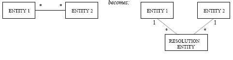
This is more general than a standard UML association class, as it solves some of the weaknesses in the association class, such as only having one association class per relationship.
Transaction model checking simply is ensuring that:
- all necessary components are represented
- all class operations are called by the manager
- indirect messages relate to the creation and deletion of links
- messages that call set-based operations have sets as targets
- consistency of guards.
Finally, model cross checking of the class and collaboration models leads to elaboration of, at least, the class model. It checks that there are enough transactions to handle the data and there is enough data to carry out the transactions. The basic checking processes are that all called operations are available in the classes and all data in guards and parameters must be available. Extra checks such as general checks, integrity checks and navigation checks could also be used.
To check there are enough transactions, you need to ensure that every class has transactions to create, delete and change the attributes of an instance, and every association has transactions to create and delete links. Therefore, for every role whose multiplicity does not include 0, any transaction that creates an instance of the opposite class must also create a link to that instance and any transaction that deletes the last or only link to the opposite class must also delete the instance of the opposite class.
Integrity checks ensure that business rules are properly expressed, and the simplest of them are the structural integrity rules imposed by the diagram, so you have to ensure that the structural integrity is correctly captured in the class model and the collaboration diagrams enforce structural integrity.
Navigation checks ensure that all possible questions can be answered by the data model. Connection traps occur when the structure looks fine, but does not yield answers to the needed navigations. Navigation checks consist of considering each of the required transactions of the system, and making sure that they can all be implemented in the system. You do need to make sure that by solving connection traps, unjustifiable closed loops are not introduced.
Quality of Information Systems
We can consider some of the quality rules for object orrientated software engineering when developing quality software for databases. We've already considered the direct mapping rule with relational databases, where just the specification language is adapted. We can also consider the small interfaces rule (data components are minimally linked), the explicit interfaces rule (integrity rules specify the dependencies between data) and the information hiding rule (physical data is hidden).
Databases
There are many different definitions of a database. Most focus on the features of the universe of discourse (what the database is holding), purpose, related sets of data, organised persistent data, shared access and central control and transactions.
Databases need not necessarily be computerised (the first ones for example were paper based), but for the context of this module, we will only consider computerised databases. Early non-computerised databases used manual catalogues and procedures, and in addition to the obvious inconveniences, there was the major problem of duplication, and there was no established database theory.
With the rise of computing in the 1970s, limited computing resources became available and database theory became developed. Databases were typically implemented in files using file handling programs, but duplications and manual checks were still needed. Maintenance was also difficult and there is very little support for security.
Moving into the 1980s, some theory became established and relational databases were introduced. Simple networks of computers became available and DBMSs are a hot topic in research.
ANSI/SPARC Architecture
The American National Standards Committee Standards Planning And Requirements Committee (ANSI SPARC) proposed a three-level architecture for the design and implementation of databases as show below:
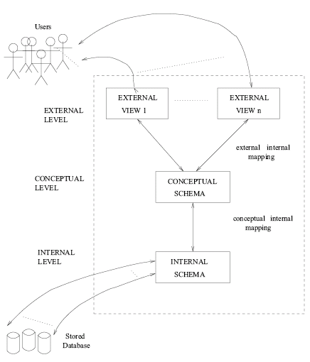
This is a theoretical model for database implementation that doesn't deal with operating systems, or the specifiation or design levels. Most good DBMSs, especially large ones, implement the SPARC architecture.
The internal level is the hidden computer storage, organised in fiile structures. The conceptual level is a model in the relevant paradigm (for this course, this is a relational model). The external level is composed of the views of the conceptual level needed by each group of users. At all the levels, we call the description of the database a schema.
The ANSI/SPARC architecture promotes insulation of data from programs, and ensures each level is independent and transparent. A DBMS that supports ANSI/SPARC should provide:
- a structure for storing data
- mapped structures for envisaging and using data
- access controls to ensure that data can only be entered and used via these structures
In ANSI/SPARC, we can consider internal mappings - the links between the architecture levels which are used to provide physical data through external views, and external mappings - which situate the DBMS in the system context (users and storage media) and provide links to the users and the computer systems.
We can consider the components of a DBMS as demonstrated in the diagram below:
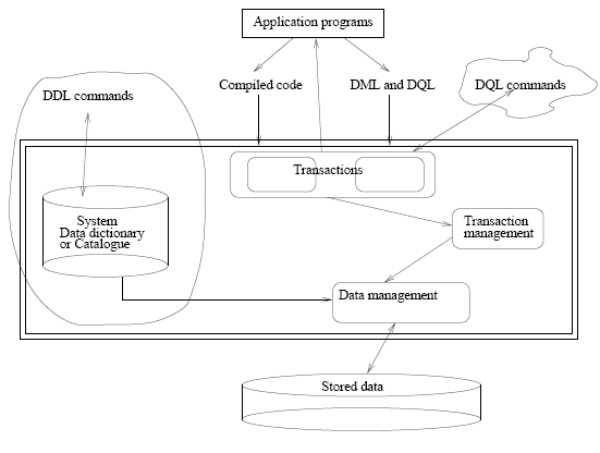
DDL (the data definition language) can be considered as an unofficial entry point to the DBMS as it provides us with direct access to the data dictionary. Most applications communicate using DML and DQL (data manipulation and data query languages). A second raw DQL approach is often used by database administrators where they need quick access to data that a transaction does not necessarily exist for. The only "official" access to the data should be through application programs using transactions.
Ultimately, the goals of a DBMS are:
- persistent storage of programs and data structures in a common format
- controlled, minimal redundancy
- representation of complex data structures (with integrity constraints)
- controlled multi-user access
- prevention of unauthorised access
- management of security features
- provision of backup and recovery facilities
Users of a DBMS
We can consider a DBMS to be used by four groups of people (roles).
- Database developers - design new database or undertake complex modifications to existing ones - typically have full access, but only on development systems
- Database administrators - involved with low-level access, responsible for granting access permissions, efficiency, modifying structure of a live database. They have constrained access to structure and wide access to data.
- Application developers - programmers of the applications that implement transactions. They are typically involved in both the development of the initial database, or can be brought in later to extend or update the system.
- End users - these use built application programs or queries to access the database to read and update data as appropriate. Typically they have tightly-controlled access rights based on their role within the organisation.
Relational Databases
Relational databases are the most widely used database paradigm, and are the basis for commercial developments in object-relational paradigms.
Relations are subsets of a cross product of domains (sets of values), and relational models are defined as collections of relations. With a relational model, we can use very abstract algebraic (relational algebra) and logic (relational calculus) languages can be used to specify transactions. With a relational DBMS, the internal and conceptual schemas, as well as the views, are defined by relations.
A relation is a set, and a table is a concrete representation of a relation - there are no duplicate rows or columns and the order of the rows and columns is irrelevant. We can consider relation intensions (the type of relation - sometimes called the schema) and relation extensions (the data that exists at a particular time).
Primary keys are used to uniquely identify tuples, and they are unique, unchanging, never null attributes, or combination of attributes. An entity integrity of the primary key is that no attribute of it takes null values.
We decide which key is the primary key by analysing single attributes for candidate keys. If there are none, we analyse combinations of attributes for more candidate keys, and then pick the minimal candidate keys (the ones that involve the least number of attributes) and choose a key using an arbritrary (but informed) decision. If there are no suitable attributes or combination of attributes, then we can define a surrogate key (one which is created with the sole purpose of being a primary key).
Relations are linked by using the primary key of one relation as a foreign key in the intension of the linked relation (this is indicated with a * and a dotted arrow to the relevant primary key, and the primary and foreign key must use the same domain). This gives us a new referential integrity constraint - the values of the foreign key in any existing extension are legitimate values of the corresponding primary key in its existing extension, or null for optional relationships.
Null values are a possible value of every domain, they are used as a place holder and can be interpreted as being irrelevant, unknown, or unknown if a value even exists. However, the last interpretation does not work in the closed loop model, where we assume that the database is a representation of the real world - we can infer things from data that is not present in the database.
There is also a problem of how to do we perform arithmetical operations on null values. In early times, inconsistent "funny" values were used (e.g., 0, 9999, etc), which in itself introduces more problems. We should try and avoid null values where possible.
To design relation intensions from the class diagrams, we create a relation intension for each class and identify primary keys. To deal with relationships, we take different approaches depending on the multiplicity:
- Many-to-many or 0..1 to 0..1 - we create a third relation comprising the primary keys
- Many-to-one - we post the primary key of the one-end class to the many-end class
- One-to-one - we add the primary key of one to the other
However, we do have a problem when it comes to handling subclasses. Subclasses do not exist in relational theory, so relations need to be used. Important concerns include participation (is every instance a member of a subclass?), disjointness (can an instance belong to more than one subclass?), transactons, and the associations in which the classes are involved.
Three ways to represent this include collapsing the hierarchy, equating inheritence to 1-to-1 relationships, or removing the supertype, but the type we choose depends on the concerns listed above.
Relational Algebra
Relational algebra is used in the design of transactions, and forms the conceptual basis for SQL. It consists of operators and manipulators, which apply to relations and give relations as a result, but do not change the actual relation in the database.
The operators come from the mathematical operators od dealing with sets:
| Relational Operator | Meaning |
|---|---|
| union(R1, R2) → R3 | R3 has all the tuples from R1 and R2 |
| difference(R1, R2) → R3 | R3 has all the tuples of R1 which are not tuples of R2 |
| intersection(R1, R2) → R3 | R3 has all the tuples that are in both R1 and R2 |
| product(R1, R2) → R3 | The intension of R3 is the concatenation of those of R1 and R2. The tuples of R3 are those of the cross product of R1 and R2 |
We can also consider the manipulators of relational algebra:
| Relational Manipulator | Meaning |
|---|---|
| restrict(R1; predicate) → R2 | R2 is a relation comprising only of the tuples of R1 for which the predicate is true |
| project(R1; predicate) → R2 | R2 is a relation comprising only the attributes of R1 specified in the predicate |
| join(R1, R2; predicate) → R3 | R3 is a relation comprising of tuples from R1 and R2 joined according to a condition on common attributes specified in the predicate |
| divide(R1, R2; predicate) → R3 | R3 is a relation formed by identifying tuples in R1 which match the values of attributes in R2, according to the predicate, and returning the values of all other attributes of the identified tuples; R3 is the relational image of R2 on R1 |
These operations can be joined to be able to give more interesting queries, e.g., "What are the numbers of the flights that go to Bangkok?" could be represented by: project(restrict(FLIGHT; Destination = Bangkok); FlightNo).
It is often simpler to represent complex queries diagramatically, such as for "What are the identifiers of the holidays that Ana has booked?":
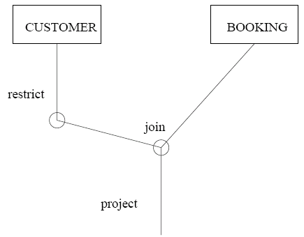
Another type of query to consider is the existential query, where we look for the existance of a connection between two relations. The solution for this is to restrict, then join and project. This is not very efficient, however, as joins and products create huge relations. A good approach to use is to get the queries correct and then think about adding projects and restricts before joining to optimise the operation. For existance between multiple relations, existantial queries can be included in one another.
In the case of universal queries, we are not interested in specific customers or packages (for example), and we can use the divide manipulator to implement these. For divide(R, S) to be well-defined, the intension of S must be a proper subset of the intension of R. The resulting relation has an intention of the attributes a of R that are not in S and an extension of the tuples t of the projection of R to a such that, for every tuple u of S, tu is in R.
Some queries can be handled as either an existential or universal query, however.
Relational algebra is not computationally complete, however (you can not write general queries), and other problems can occur - such as finding out the number of tuples in a relation.
Relational Calculus
See LPA for
predicate calculus
Relational calculus is an alternative to relational algebra and forms another conceptual basis to SQL. We can think of relational algebra as being prescriptive (how - a procedural style similar to programming languages), whereas relational calculus can be thought of as descriptive (what - a nonprocedural style based on predicate calculus). Which form you use is a matter of style.
The relational algebraic expression project(restrict(FLIGHT; Destination = Bangkok); FlightNo) can be expressed as relational calculus using a set comprehension: f : FLIGHT f.FlightNo where f.Destination = Bangkok, or perhaps the more familiar notation { f : FLIGHT | f.Destination = Bangkok ∧ f.FlightNo }.
The basic syntax of relational calculus is tuple-specification where predicate. The tuple specification and the predicate use range variables, and the tuple specification is a list of range variables and attribute selections and the predicate is over the range variables in the tuple specification. The result of this is a relation composed of the tuples of the form tuple-specification such that predicate is true.
Existential queries in relational calculus are implemented using a range variable for the target relation, an existential quantification, and one quantified variable per relation from the anchor up to, but not including the target relation and equalities to establish the starting points and links.
To do universal queries, we use a universal quantifier with a range variable for the target relation, a quantified range variable for the anchor relation and a quantified predicate, which is an existential query to establish a connection between the anchor and the target.
We do however have the same problems as we had with relational algebra, where general search algorithms can not be implemented - this is due to a restriction in predicate calculus.
A variant of relational calculus is domain calculus, where predicate logic is defined over domains, rather than relations.
In conclusion, relational calculus is useful for defining relations and for optimisation (a huge number of algebraic laws exist). For the evaluation of language, relational calculus is relationally complete, and relational algebra is a convenient target to implement the calculus, and an algorithm exists which can transform any calculus expression into an algebra expression.
Normalisation
Normalisation is a technique to eliminate duplicated data and unnecessary attributes. It is applied during the design stage and ensures that all relations comply with restrictions imposed by normal forms - a succession of rules. Normalisation helps reveal relations and avoid inconsistency during transactions.
The result is not necessarily efficient (e.g., duplicated data might be used to speed up a search), and any changes in the physical design for efficiency reasons should be recorded.
Dependence among attributes needs to be controlled, and anomalous results when inserting, updating or deleting data need to be reduced, as well as eliminating spurious tuples when joining relations. Dependencies such as one value determining another (functional dependence) are not recorded in the design, which is a problem.
The need for normalisation was proposed by Codd very early after he recognised a need for a technique to remove dependencies. The first three levels of normalisation were suggested in 1972 and subsequently, Boyce and Codd added a further level (BCNF). Other research has produced further forms, although these are concerned with dependencies other than those the first three and BCNF (such as between tuples, relations and their projections), which are concerned with the dependencies between attributes of a tuple.
An attribute B is functionally dependent on another attribute, A, if, at any time, knowing the value of A uniquely determines the value of B. We write this as A → B, where A and B can be lists of attributes.

Functional dependencies exist between the primary key and other attributes, and normalisation removes any other functional dependency. To identify the functional dependencies, we use the domains and integrity constraints, rather than a particular extension - which can only show the absence of a functional dependency. In relational databases, we can consider a universal relation, which is a join of all relations in a database, and attribute names are prefixed by the name of their original relation.
Given a set of functional dependencies, we can infer others, known as Armstrong's axioms:
- Reflexivity - if Y ⊆ X, then X → Y
- Augmentation - if X → Y, then XZ → YZ
- Transitivity - if X → Y and Y → Z, then X → Z
- Composition - if X → Y and X → Z, then X → YZ
- Decomposition - if X → YZ, then X → Y and X → Z
- Pseudo-transivity - if X → Y and WY → Z, then WX → Z
This is sound and complete, and only reflexivity, augmentation and transitivity are enough. Any functional dependencies satisfied by the axiom of reflexivity are considered trivial, and do not say anything special about the application.
Derived attributes represent required calculations (e.g., age from birth date) and are recorded in the data dictionary. They characterise a functional dependency, but are not part of the relational model and prevent full normalisation.
To start normalisation, you need to determine non-trivial functional dependencies and at the end of each level of normalisation, relations should be presented complete with their primary and foreign keys.
First Normal Form
The first normal form (1NF) is concerned with the internal structure of attributes and domains need to be clearly defined.
A relation in 1NF has no set-valued attributes; all its attributes contain only atomic values from their domains.
An attribute can be a set if sets are values of the domain, otherwise a new relation is needed.
Second Normal Form
The second normal form (2NF) requires that attributes are properly dependent on the primary key. It is a concern for any relation with a multi-attribute primary key.
A relation is in 2NF if, and only if, it is in 1NF, and every non-prime attribute is fully functionally dependent on the primary key.
A non-prime attribute is one which is not part of any candidate key. We can say that A is functionally dependent on B: B → A, but not C → A for any C ⊂ B.
Foreign keys then allow the original data structure to be recreated from the normalised relations if necessary.
Third Normal Form
The third normal form (3NF) is concerned with mutual dependencies of attributes that are not in the primary key.
A relation is in 3NF if, and only if, it is in 2NF, and no non-prime attributes are transitively dependent on the primary key.
A is transitively dependent on B if there is a C such that B → C and C →, and C is not a candidate key.
Any internally dependent attributes should be extracted to a seperate relation for this stage of normalisation to be applied.
Boyce-Codd Normal Form
Boyce-Codd Normal Form (BCNF) applies to relations that have two or more candidate keys that overlap and is stricter than 3NF; every relation in BCNF is in 3NF, but a relation in 3NF may not be in BCNF. In other cases, 3NF will be enough.
A relation is in BCNF if, and only if, whenever an attribute A is functionally dependent on B, then either B contains all the attributes of a candidate key of R, or A is in B.
One way of normalising to BCNF is to extract attributes in the offending dependency to a new relation.
Algorithms for normalisation work by decomposing the non-normalised relations into two or more normalised relations using the methods explained above. Some authors propose the use of normalisation through decomposition as the central technique to design a relational model, starting from the universal relation and the functional dependencies. This preserves dependencies, as all dependencies of the universal relation can be inferred from the dependencies that only involve attributes of a single relation, and this is reasonably easy to enforce. This approach is not often taken in practice, though.
We can also consider the property of lossless-join, where decomposed relations can always be joined back using the join operator of relational algebra on the primary and foreign keys, to exactly the contents of the original relation, and no spurious tuples should be introduced by the join.
It is always possible to normalise a relation to 3NF to obtain a collective of relations that preserve depenency and the lossless-join property, and it is always possible to normalise a relationship to BCNF and maintain lossless-join, however it is not always possible to obtain relations that satisfy all the properties. When this occurs, the problem should be recorded and a compromise made.
SQL
SQL (Structured Query Language) is the most popular relational database language. It implements both a DDL and a DML and concerns itself with the creation, update and delation of relations and properties based on relational algebra and calculus. It is typically included in host applications, or conventional computer programs.
SQL is based on SEQUEL (Structured English QUEry Langauge) which was developed by IBM in the 1970s for System R. In 1986, ANSI developed a standardised version of SQL based on IBM's SEQUEL, and in 1987, ISO also released a version, which was updated with integrity enhancements in 1989, and then again in 1992 (SQL-92) and 2000 (SQL-99, sometimes referred to as SQL-3). The current version of SQL is SQL-2003 and adds object-relational features and XML, etc...
There are many variations and specialised versions of SQL, e.g., ORDBMS SQL for object-relational products was marketed by DB2, Oracle and Informix, Geo-SQL is used in various GIS products, and TSQL2 is a temporal query language much cited in research. They do all have a common core, but other varients include direct SQL and embedded SQL, differences in access privileges and concurrency and not stored SQL, which includes the usual control commands.
Tables
In SQL, tables look like relations, but are not actually sets as duplication can occur. Duplications can be removed, but the column order will always matter. There are three types of tables, base tables, views and result tables. Base tables are persistent, normalised relations that are often defined by metatables; views are derived from the base table, or other views (note, these are different from the views of the ANSI/SPARC architecture) and there is a deal of controversy when discussing updates. Finally, result tables are transient and hold the results of queries - these can be saved by making them a view.
To implement a relational structure, the main activity is creating the base tables. We need to discover the data domains that are available in the DBMS and then map the logical domains to the physical domains and record the decisions made to do this. We need to perform a final check that integrity and normalisation still holds and then use the SQL CREATE command to implement the relations.
The first step is to use CREATE SCHEMA schema_name to create the database all our relationships exist in. The second step is to create the tables themselves using CREATE TABLE table_name(attr1 type1 options1, ..., attrn typen optionsn, further_options).
Integrity Constraints
Integrity constraints can be implemented using the PRIMARY KEY key_name statement in the further_options part of the CREATE TABLE command, additionally, foreign keys can be implemented using CONSTRAINT constraint_name FOREIGN KEY (key_name) REFERENCES table_name in the further_options part.
Data domains can also be defined using the CREATE command - CREATE DOMAIN domain_name type DEFAULT d CHECK expression. Additionally, checks can be declared on the whole table with the CHECK command. A UNIQUE statement can be used for alternative simple candidate keys. Checks can be deferred.
When integrity constraints involve more than one table, we can use the CREATE ASSERTION command - CREATE ASSERTION assertion_name expression. Assertions are checked at the end of every transaction, so they are more costly in performance terms than CHECK.
Additionally, we can use triggers to implement integrity constraints. Triggers are associated to one table and to an update operation. It does not avoid the update, but it can undo one that has been done. They take action when a specified condition is satisfied, e.g., CREATE TRIGGER trigger_name BEFORE UPDATE OF table_name REFERENCING OLD ROW AS old_tuple NEW ROW AS new_tuple FOR EACH ROW WHEN expression SET expression.
Using ON DELETE and ON UPDATE, we can have flexibility in handling referential integrity, but we need to consider whether or not we really need that. We can use cascades to handle mandatory association with the CASCADE command, so we have enfored referential integrity.
Views
As queries and result tables are lost, we can use CREATE VIEW to associate a name with a particular query, e.g., CREATE VIEW view_name AS expression.
SQL Statements
Now we can start considering the basic SQL commands:
- INSERT INTO table_name(attr1, ..., attrn) VALUES(value1, ..., valuen)
- DELETE FROM table_name WHERE predicate
- UPDATE table_name SET attr1=value1, ..., attrn=valuen, (attr1, ..., attrn) = subquery WHERE predicate
- SELECT DISTINCT attr1,...,attrn FROM table1,...,tablen WHERE predicate GROUP BY attr1,...,attrn HAVING func1,...,funcn ORDER BY attr1 DESC/ASC, ..., attrn DESC/ASC
SELECT is the most used command, and it can be used to write statements based on relational algebra and calculus. Using a simple SELECT command you can project, product and restrict, e.g., project(restrict(product(table1, table2); predicate); attr1, attr2) can be translated in to SQL as SELECT attr1,attr2 FROM table1,table2 WHERE predicate. The predicate in SQL is used to select attributes or tuples for which the predicate is true. The predicates are built from comparators and logical connectives, e.g., Attr1 [NOT] BETWEEN Attr2 AND Attr3, Attr1 IS [NOT] NULL, Attr [NOT] LIKE pattern, etc...
Using IN conditions in the predicate allows nesting of queries e.g., SELECT * FROM flight WHERE flightno IN (SELECT flight FROM holpackage) - this is computationally expensive, however, as the nested query is evaluated once for each candidate tuple of the outer query. The nested query refers to an attribute of a relation in the outer query - these types of query are called correlated queries.
The EXISTS operator can be used in a predicate to check the existance (non-null value) of another query, e.g., SELECT DISTINCT custno FROM booking first WHERE hpackid='Cultural' AND EXISTS SELECT custno FROM booking second WHERE second.custno = first.custno and second.hpackid='Football'.
We can also use aggregate functions in our select query, e.g., SELECT hpackid, COUNT DISTINCT custno FROM booking GROUP BY hpackid HAVING COUNT DISTINCT > 2.
In addition to our SELECT - FROM - WHERE project - product - restrict form of an SQL query, we can also use the explicit operators UNION, INTERSECT and EXCEPT for union, intersection and difference respectively. Additonally, there is also an explicit JOIN operator with several extensions, and division has been replaced by the facility to consider predicates involving relations. To force our queries to return sets, we must qualify the SELECT command with the DISTINCT option.
Joins exist in many forms, with the most basic being the relational algebra, or inner, join. This can be expressed as either SELECT * FROM table1,table2 WHERE table1.attr1 = table2.attr3, or in the form of SELECT * FROM table1 INNER JOIN table2 USING (attr1).
If an attribute of one or both tables are required, whether they are linked to a tuple of the other table or not, outer joins can be used. The syntax is the same as for the JOIN command above, except with INNER being replaced by the type of join being used. LEFT OUTER JOIN is when all the tuples of the table to the left of the JOIN are required, and similarly for RIGHT OUTER JOIN, all the tuples to the right of the JOIN are included. For completeness, there is also FULL OUTER JOIN, which includes all the tuples from both tables. Any values that are blank in the other table after the join are left as null.
SQL only supports existential quantification using the EXISTS qualifier, and not universal quantification, however we can use the following rule to map a universal query to an existential one: (∀x : T ∧ p) ≡ ¬(∃x : T ∧ ¬p).
SQL is used with other programming languages, so we need to consider how to distinguish SQL commands from our standard program and how to map data from the database to host-program data structures and how to determine the start and end of a transaction.
One implementation in C is the call level interface specification, which is where most of the database queries are handled in the preprocessor. Other languages, such as Java, PHP and modern implementations of C use the core library and drivers to access it (e.g., ODBC or JDBC).
CLI statements in C look like: EXEC SQL query. Shared variables are declared between EXEC SQL BEGIN DECLARE SECTION and EXEC SQL END DECLARE SECTION, and then are referenced in the query by prefixing it with a colon, e.g., EXEC SQL SELECT count(custno) INTO :numcust FROM booking. We need to make sure that we have correct data types (or weird things will happen when we start casting), and these need to be checked.
When we are dealing with multiple tuples, it is often easier to use a CURSOR, which is declared as EXEC SQL DECLARE ptr CURSOR FOR query, and then EXEC SQL OPEN ptr, FETCH FROM ptr into :var (repeated as many times as necessary) and then finally EXEC SQL CLOSE ptr.
Transactions in C are started by an EXEC SQL CONNECT host username IDENTIFIED BY password command and then either an EXEC SQL COMMIT command, or EXEC SQL ROLLBACK. Either way, the connection should then be released.
In other languages, which are based on an API (such as the JDBC in Java or mysqlclient in C), distinguishing SQL commands is not an issue as it is not compiled in advance. However, a more flexible and complex approach of processing results is needed. In JDBC, we can use commands such as DriverManager.getConnection(...), creating a statement is done with stmt = conn.createStatement(), and then the statement is executed using rs = stmt.executeQuery(...). The result set rs is then processed with command such as rs.getInt(i), rs.getString(i), etc. Finally, the result set is closed with stmt.close() and the connection closed using conn.close().
Security
When designing security measures for databases, we should start from the assumption that agents (people) intend harm, this contrasts with safety, which exists to prevent accidents (although the two can complement each other in areas).
In databases, security stems from the need for military and commercial secrecy, and was typically implemented using encryption and physical isolation, however, with the rise of multi-user databases, this is not feasible. With the advent of Internet connected databases, there is even less control over who might try to access the database, the number and type of these concurrent accesses and what parts of the database can be accessed.
Threats are potential entries that could be used to cause harm, whereas an attack is the exploitation of a threat. Possible threats could come from authorised users abusing their privileges and the possibility of unauthorised access. The potential consequences of a successful attack include a breach of security, integrity and availability. One of the key tasks in database security is to identify threats. Countermeasures to attacks include access control, inference control, flow control and encryption.
Good database systems should have a security policy and mechanisms in place to implement the security policy. The security policy typically consists of a set of high-level guidelines and requirements based on user needs, the installation environment and any institutional and legal constraints. The mechanisms are a set of functions that apply the security policy and can be implemented in hardware, software and human procedures. Mechanisms could either be mandatory controls which can not be overridden and discretionary controls, which allows privleged users to bypass restrictions.
To capture mechanisms that address policies, we have objects (entities that need to be protected) classified by a scale of security. Subjects request access to objects, and they need to be controlled. Subjects are classified by a scale of truth.
Military Model
In the military model of security, we have all controls as mandatory, and confidentiality is the number one concern. In this model, the objects are the values of attributes and subjects are the database users. The classic secrecy classification of objects is top secret, secret and unclassified, and subjects are similarly classified. This determines which categories of subject can access which categories of object.
Security should be considered early on in the database development process, before the specification stage. General things that should be considered include questions such as:
- How private is the data?
- How robust and rigorous does the subject need to be?
- Are the requirements the same for all data?
- What is the security policy?
- What is the appropriate model to be applied?
- Does the development need tailoring?
If we know the DBMS at this stage, then the facilities of that should be considered as part of the analysis.
During the specification stage, we should consider access control. Groups who have common access rights need to be identified and assigned to roles, and then transactions should be annotated with access requirements. For each class, roles should be assigned responsibilities for creation, deletion and manipulation of data. When designing verification plans, testing should include cases to check that security is enforced and for each transaction that an intersection of roles is responsible for the constituent operations.
If any inconsistency does come up in the consultation (e.g., someone does not have the roles required to run all of the parts of a transaction - i.e., they do not have access to a class that needs data deleting when a transaction requires that data to be deleted), then further consultation with the client is needed, and it can often be worked around with, for example, views.
Relational theory contains nothing about security in databases, however SQL has implemented some access control facilities using the GRANT statement.
SQL
In SQL, users are subjects and there is no classification of objects, which can be tables, attributes or domains. Privileges are expressed using DML commands such as GRANT and REVOKE, which grants permission for an object and a privilege to a subject. SQL only supports discretionary control.
The GRANT command has the syntax of GRANT privilege ON object TO subject, with privilege is a command, such as SELECT, UPDATE, etc... More control can be used by specifying columns in the privilege, e.g., UPDATE(column) would only allow updates on that column in the table. The use of views allows an even finer control over access, limiting access to certain fields, or to a certain time using the CURRENT_TIME() command in the WHERE clause of the view.
To implement this, support is needed from the host programming language, the DBMS and the OS. Good practice is to record the roles in a metatable.
Concurrency
For more information,
see Transactions in NDS.
When dealing with transactions, the introduction of concurrency into the system can bring efficiency gains, however the DBMS must ensure that integrity is not compromised by this. The safest route is sequential execution, but this is highly inefficient, so we need to introduce some form of transaction management.
We can consider transactions as a series of database operations that together move the database from one consistent state to another, although the database may be inconsistent at points during the transaction execution. It is desirable for transactions to exhibit the ACID properties to enforce this integrity when concurrency is involved. The ACID properties are:
- Atomicity - all steps must be completed before changes become permenant and visible, and if completion is not possible, then we must fail and updates are undone
- Consistency - transactions must maintain validity
- Isolation - transactions must not interfere with each other
- Durability - it must be possible to recover from system crashes
Lost Update Problem
The lost update problem is an interference problem, caused by a lack of atomicity resulting in an inconsistent database. e.g.,, if we have two concurrent executions of a Transfer transaction for moving money in a bank from an account A1 and both transactions read the current value before the other has updated, then the money deducted from A1 will only be that of the last transaction to commit, rather than the complete amount.
Uncommitted Dependency Problem
This is another interference problem causing by a lack of atomicity and resulting in an inconsistent database. If a transaction T2 starts and completes whilst a transaction T1 is running, and then T1 fails and rolls back, the result of the transaction of T2 will be lost.
Inconsistent Analysis
If a transaction reads an uncommitted update from another transactions at a point when the second transaction causes the database to be in an inconsistent state, then the first transaction is said to have performed an inconsistent analysis, even if both transactions successfully commit.
Schedulers
To work around this problem, the DBMS implements a scheduler, which orders the basic operations for efficient use of the CPU and to enforce isolation - scheduling should be serialisable.
Two different scheduling algorithms including time stamping, where the start time of a transaction is recorded, and the time is used to solve conflicts - policy may dictate whether priority is given to the older or younger transaction. Optimistic scheduling assumes that conflicts are rare, so all transactions are carried out on memory, and the possibility of conflict is analysed before committal.
Locking
Locking works by placing locks on the data accessed by transactions - complete isolation is not needed. The granuality for the lock depends on the transaction, e.g., the whole database for batch processes, a table, a page (this is what is most frequently used by multi-user DBMSs), row (this has a high overhead) or an individual field (not often implemented).
We can consider binary locking, where an object is in two states, either locked or unlocked, however this is too restrictive, or we can consider shared (S for read-only operations) and exclusive (X for write operations) locks. This does have a slightly increased overhead, however.
| Lock held by transaction 1 | |||
| X | S | ||
|---|---|---|---|
| Lock requested by transaction 2 | X | denied | denied |
| S | denied | granted | |
The two-phase locking protocol guarantees serialisability. All locks that are needed are obtained before any locks are released, this means we can categorise a transaction in to two phases, a growing phase (acquiring locks) and a shrinking phase (releasing locks).
To avoid deadlock, we can use various methods, such as prevention to abort when a lock is not available, detection using timeout and kill one of the transactions in deadlock, and avoidance, which gets all needed locks at once.
SQL
When starting a transaction, we can set the transaction type and the isolation level in SQL: SET TRANSACTION type ISOLATION LEVEL level, where the transaction types are READ ONLY, so no updates can be performed by the transaction, and READ WRITE, where updates and reads are permitted. This definition of transaction types prevents updates without proper locks and he isolation level defines the policy for the use of locks. All locks are released at COMMIT or ROLLBACK. The behaviors of the isolation levels are shown in the table below:
| X locks on tuples | S locks on tuples | X and S locks on predicates | Description | |
|---|---|---|---|---|
| READ UNCOMMITTED | N/A (read-only) | no | no | No locks, and can only be used on READ ONLY transactions. Lost update is not an issue, but uncommitted dependency and lost analysis are still problems. |
| READ COMMITTED | yes | no | no | Uses X locks, and it can read data that is not locked, using a short S lock. Uncommitted dependency is solved, but Scholar's lost update (a variant of lost update) and inconsistent analysis are still possible. |
| REPEATABLE READ | yes | yes | no | This uses X and S locks, but has a problem of phantom records. Locks are applied to tuples. |
| SERIALIZABLE | yes | yes | yes | This uses predicate locking based on the WHERE clauses of SELECT, UPDATE and DELETE, and has no concurrency problems. |
Recovery
We need to be able to restore the database to a valid state in case of failure - that is, enforce the durability aspect of the ACID properties. Most DBMSs are expected to provide some form of recovery mechanism, and most common mechanisms involve some level of redundancy, involving recovery logs and backups. Recovery issues we need to consider include system recovery, media recovery and system committal and rollback.
Transactions typically operate on the main memory buffers and are intermittently written to disk - this process is controlled jointly by the DBMS and the operating system. Updates are stored, and a log. The log stores the start of transactions, and then an entry for each update that contains enough information to be able to undo or redo the update finally with a commit. The log is essentially a database itself, and care should be taken with it as it is invaluable in case a recovery needs to be made with it.
When a write to disk occurs, the OS proceeds as usual, and at commit time, the commit is recorded in the log which is then updated first (the write-ahead log rule) and then a forced write of the log to disk occurs. This means that the log and the updates on disk may be out of phase. Checkpoints are used to force the write of data to disk.
At a checkpoint, all executing transactions are suspended, and all dirty buffer pages are written to disk. A recording of the checkpoint is made in the log, with a listing of the transactions that were active at the time of the checkpoint. The log is then written to disk and the log buffer reinitialised, and transactions unsuspended.
The recovery procedure itself is automatically initiated by the system restart. The basic procedure is to create two transaction lists, an UNDO list which contains all active transactions at the last checkpoint and then a REDO list, which is initally empty. The section of the logfile after the last checkpoint is then analysed to update the UNDO and REDO lists. Log files are parsed from top to bottom, and when a transaction is started, it is added to UNDO and when a commit is found, the transaction is moved to REDO. The logfile is then run from bottom to top to undo - this is backwards recovery - and then it is run from top to bottom to redo - forward recovery.
Recovery is implemented in SQL using intermediate savepoints which are equivalent to intermediate COMMIT points. Updates are not visible until after a savepoint, which makes partial rollbacks possible. The syntax for savepoints is simple: SAVEPOINT name, ROLLBACK TO name and RELEASE name.
In the event of a disk failure, the database and the log file are unreliable, so restoration has to be done from a backup. There is no need to undo anything as backups are made when the database is in a consistent state. Backup procedures are supported by DBMSs and work by generating consistent images of the database - a full backup. Log files (incremental backups) are stored between backups to ease the recovery process. There will always be losses in this case, however - and handling these inevitable losses are an application dependent issue that is solved by management processes.
For system commital and rollback (especially in distributed systems), all managers need to be coordinated, and one manager will have a system coordinator function. A two-phase commit protocol is used to implement system commital and rollback. The first phase is to prepare and send your commits to the system coordinator, all managers are instructed to commit and logs are written and responses collected. The second phase is to commit, where the system coordinator evaluates and records the results of the other managers and then makes the decision for each manager to make the final commit or rollback. This methods has to be used when transactions involve multiple databases.
Distribution
Distributed databases typically consist of logically related data, but they are no longer centralised - the database is broken into fragments. Management is still central, which leads to a degree of transparency in the database system. The distributed database shares a common universe of discourse.
Distributed databases can afford us efficiency, reliability, and allow us to decentralise a business. Server farms consisting of many generic servers are now common, as opposed to purchasing a large mainframe. With the rise of fast networks and the acceptance of the Internet, distributed databases are now a common reality.
With distributed databases, we can have data where it is needed, with a more flexible growth route and a reduced risk of single point-of-failure, however management and control (the duplication ghost) adds additional complexity, and considerations need to be made for increased security threats and storage requirements. There are still no standards for distributed DBMSs, and in reality there is a long way to go to perfect this area of database theory.
A distributed DBMS keeps track of local and distributed data and performs query optimisation based on the best access strategy. Most DDBMSs provide an enhanced security, concurrency and recovery facility, as well as enhanced transaction management to decompose access requests.
The components of a DDBMS include computer workstations for the data and the clients, network hardware and software and then in the clients, a transaction processor and data manager are required. Both data and processing can happen either at a single or multiple sites with a distributed system, and a certain amount of heterogeneity is supported by most DDBMSs.
DDBMS Architecture
The distributed DBMS architecture has five levels:
- Local schema
- Component scheme, in a common model
- Export schema, data that is shared
- Federated schema, global view
- External schema, this is the external level of ANSI/SPARC
Transparency is required so that the end user feels that they are the only user of local data. Distribution transparency works on the principles of fragmenation, location and local mapping. SQL supports a special NODE clause to specify the location of a fragment and to implement local mapping. Updates on duplicates also become the responsibility of the programmer. For transaction transparency, a two-phase commit protocol is used, and we also have to consider failure transparency, performance transparency (query optimisation) and heterogeneity transparency.
Design Considerations
When designing a distributed database, the same issues apply, but we have to consider the extra issues of data fragmentation, replication of fragments and the location of fragements and schemas. Data fragmentation is designed using a fragmentation schema which divides relations into logical fragments, and allows whole relations to be recreated using unions and joins. A replication schema can be used to define the replication of fragments and an allocation schema is used to define the locations. A global directory is required to hold all of these schemas.
Different strategies can be used for data fragmentation, we can either fragment horizontally, where subsets of tuples are distributed and we have a set of disjoint subsets, or we can fragment vertically, where projections are distributed and the primary key is replicated. Fragements therefore must all have the same number of rows. It is also possible to mix these strategies.
Data replication works by replicating the individual fragments of the database. With replication, we can enhance data availability and response time, as well as reducing communication and query costs. Replication works off the mutual consistency rule, where all copies are identical - updates are performed in all sites. With replication, there is an overhead in transaction management, as we have a choice of copy to access, and synchronised update. Replication can greatly ease recovery.
Query optimisation can also be used to minimise data transfer. The choice of processing site is based on estimates, and most DDBMSs provide a semijoin operator, which reduces the number of tuples before transferring by combining a project() with a join().
For election algorithms,
see NDS.
Distributed concurrency is based on an extension of the locking mechanism. A coordinator site exists which associates locks with distinguished copies at a primary site (with or without a backup site) and a primary copy. Coordinators are chosen using an election process, or a voting method.
Codd specified a set of twelve commandments for distributed databases - although none are implemented in modern DDBMSs, like the similar commandments for relational systems, they provide a framework for explanation and evaluation.
- Local site independence
- Central site independence
- Failure independence
- Location transparency
- Fragmenation transparency
- Replication transparency
- Distributed query processing
- Distributed transaction processing
- Hardware independence
- Operating system independence
- Network independence
- Database independence