Languages
For more detail
see TOC.
Languages are a potentially infinite set of strings (sometimes called sentences, which are a sequence of symbols from a given alphabet). The tokens of each sentence are ordered according to some structure.
A grammar is a set of rules that describe a language. Grammars assign structure to a sentence.
An automaton is an algorithm that can recognise (accept) all sentences of a language and reject those which do not belong to it.
Lexical and syntactical analysis can be simplified to a machine that takes in some program code, and then returns syntax errors, parse trees and data structures. We can think of the process of description transformation, where we take some source description, apply a transformation technique and end up with a target description - this is inference mapping between two equivalent languages, where the destination is a machine executable.
Compilers are an important part of computer science, even if you never write a compiler, as the concepts are used regularly, in interpreters, intelligent editors, source code debugging, natural language processing (e.g., for AI) and for things such as XML.
Throughout the years, progress has been made in the field of programming to bring higher and higher levels of abstraction, moving from machine code, to assembler, to high level langauges and now to object orrientation, reusable languages and virtual machines.
Translation Process
LSA only deals with the front-end of the compiler, next year's module CGO deals with the back-end. The front-end of a compiler only analyses the program, it does not produce code.
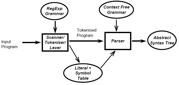
From source code, lexical analysis produces tokens, the words in a language, which are then parsed to produce a syntax tree, which checks that tokens conform with the rules of a language. Semantic analysis is then performed on the syntax tree to produce an annotated tree. In addition to this, a literal table, which contains information on the strings and constants used in the program, and a symbol table, which stores information on the identifiers occuring in the program (e.g., variable names, constant names, procedure names, etc), are produced by the various stages of the process. An error handler also exists to catch any errors generated by any stages of the program (e.g., a syntax error by a poorly formed line). The syntax tree forms an intermediate representation of the code structure, and has links to the symbol table.
From the annotated tree, intermediate code generation produces intermediate code (e.g., that suitable for a virtual machine, or pseudo-assembler), and then the final code generation stage produces target code whilst also referring to the literal and symbol table and having another error handler. Optimisation is then applied to the target code. The target code could be assembly and then passed to an assembler, or it could be direct to machine code.
We can consider the front-end as a two stage process, lexical analysis and syntactic analysis.
Lexical Analysis
Lexical analysis is the extraction of individual words or lexemes from an input stream of symbols and passing corresponding tokens back to the parser.
If we consider a statement in a programming language, we need to be able to recognise the small syntactic units (tokens) and pass this information to the parser. We need to also store the various attributes in the symbol or literal tables for later use, e.g., if we have an variable, the tokeniser would generate the token var and then associate the name of the variable with it in the symbol table - in this case, the variable name is the lexeme.
Other roles of the lexical analyser include the removal of whitespace and comments and handling compiler directives (i.e., as a preprocessor).
The tokenisation process takes input and then passes this input through a keyword recogniser, an identifier recogniser, a numeric constant recogniser and a string constant recogniser, each being put in to their own output based on disambiguating rules.
These rules may include "reserved words", which can not be used as identifiers (common examples include begin, end, void, etc), thus if a string can be either a keyword or an identifier, it is taken to be a keyword. Another common rule is that of maximal munch, where if a string can be interpreted as a single token or a sequence of tokens, the former interpretation is generally assumed.
For revision of
automata,
see MCS
or lecture notes.
The lexical analysis process starts with a definition of what it means to be a token in the language with regular expressions or grammars, then this is translated to an abstract computational model for recognising tokens (a non-deterministic finite state automaton), which is then translated to an implementable model for recognising the defined tokens (a deterministic finite state automaton) to which optimisations can be made (a minimised DFA).
Syntactic Analysis
Syntactic analysis, or parsing, is needed to determine if the series of tokens given are appropriate in a language - that is, whether or not the sentence has the right shape/form. However, not all syntactically valid sentences are meaningful, further semantic analysis has to be applied for this. For syntactic analysis, context-free grammars and the associated parsing techniques are powerful enough to be used - this overall process is called parsing.
In syntactic analysis, parse trees are used to show the structure of the sentence, but they often contain redundant information due to implicit definitions (e.g., an assignment always has an assignment operator in it, so we can imply that), so syntax trees, which are compact representations are used instead. Trees are recursive structures, which complement CFGs nicely, as these are also recursive (unlike regular expressions).
There are many techniques for parsing algorithms (vs FSA-centred lexical analysis), and the two main classes of algorithm are top-down and bottom-up parsing.
For information about
context free grammars,
see MCS.
Context-free grammars can be represented using Backus-Naur Form (BNF). BNF uses three classes of symbols: non-terminal symbols (phrases) enclosed by brackets <>, terminal symbols (tokens) that stand for themselves, and the metasymbol ::= - is defined to be.
As derivations are ambiguous, a more abstract structure is needed. Parse trees generalise derivations and provide structural information needed by the later stages of compilation.
Parse Trees
Parse trees over a grammar G is a labelled tree with a root node labelled with the start symbol (S), and then internal nodes labelled with non-terminals. Leaf nodes are labelled with terminals or ε. If an internal node is labelled with a non-terminal A, and has n children with labels X1, ..., Xn (terminals or non-terminals), then we can say that there is a grammar rule of the form A → X1...Xn. Parse trees also have optional node numbers.
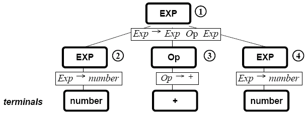
The above parse tree corresponds to a leftmost derivation.
Traversing the tree can be done by three different forms of traversal. In preorder traversal, you visit the root and then do a preorder traversal of each of the children, in in-order traversal, an in-order traversal is done of the left sub-tree, the root is visited, and then an in-order traversal is done of the remaining subtrees. Finally, with postorder traversal, a postorder traversal is done of each of the children and the root visited.
Syntax Trees
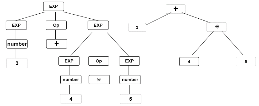
Parse trees are often converted into a simplified form known as a syntax tree that eliminates wasteful information from the parse tree.
At this stage, treatment of errors is more difficult than in the scanner (tokeniser), as the scanner may pass problems to the parser (an error token). Error recovery typically isolates the error and continues parsing, and repair can be possible in simple cases. Generating meaningful error messages is important, however this can be difficult as the actual error may be far behind the current input token.
Grammars are ambiguous if there exists a sentence with two different parse trees - this is particularly common in arithmetic expressions - does 3 + 4 × 5 = 23 (the natural interpretation, that is 3 + (4 × 5)) or 35 ((3 + 4) × 5). Ambiguity can be inessential, where the parse trees both give the same syntax tree (typical for associative operations), but still a disambiguation rule is required. However, there is no computable function to remove ambiguity from a grammar, it has to be done by hand, and the ambiguity problem is undecidable. Solutions to this include changing the grammar of the language to remove any ambiguity, or to introduce disambiguation rules.
A common disambiguation rule is precedence, where a precedence cascade is used to group operators in to different precedence levels.
BNF does have limitations as there is no notation for repetition and optionality, nor is there any nesting of alternatives - auxillary non-terminals are used instead, or a rule is expanded. Each rule also has no explicit terminator.
Extended BNF (EBNF) was developed to work around these restrictions. In EBNF, terminals are in double quotes "", and non-terminals are written without <>. Rules have the form non-terminal = sequence or non-terminal = sequence | ... | sequence, and a period . is used as the terminator for each rule. {p} is used for 0 more occurrences of p, [p] stands for 0 or 1 occurances of p and (p|q|r) stands for exactly one of p, q, or r. However, notation for repetition does not fully specify the parse tree (left or right associativity?).
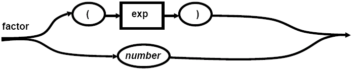
Syntax diagrams can be used for graphical representations of EBNF rules. Non-terminals are represented in a square/rectangular box, and terminals in round/oval boxes. Sequences and choices are represented by arrows, and the whole diagram is labelled with the left-hand side non-terminal. e.g., for factor → (exp) | "number" .
Semantic Analysis
Semantic analysis is needed to check aspects that are not related to the syntactic form, or that are not easily determined during parsing, e.g., type correctness of expressions and declaration prior to use.
Code Generation and Optimisation
Code generation and optimisation exists to generally transform the annotated syntax tree into some form of intermediate code, typically three-address code or code for a virtual machine (e.g., p-code). Some level of optimisation can be applied here. This intermediate code can then be transformed into instructions for the target mahcine and optimised further.
Optimisation is really code improvement, e.g., constant folding (e.g., replace x = 4*4 with x = 16), and also at a target level (e.g., multiplications by powers of 2 replaced by shift level instructions).
T-Diagrams
T-diagrams can be used to represent compilers, e.g.,
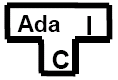
This shows an Ada compiler, written in C that outputs code for the Intel architecture. Cross compilers can also be represented, e.g.,
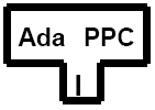
This shows an Ada compiler for PowerPC systems that is written for the Intel architecture.
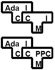
T-diagrams can be combined in multiple ways, such as to change the target language:
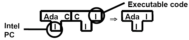
Or to change the host language, e.g., to compile a compiler written in C or to generate a cross-compiler:
Bootstrapping
The idea behind bootstrapping is to write a compiler for a language in a possibly older version or a restricted subset of the language. A "quick and dirty" compiler is then written for that language that runs on some machine, but in a restricted subset or older version.
This new version of the compiler incorporates the latest features of the language and generates highly efficient code, and all changes to the language are represented in the new compiler, so this compiler is used to generate the "real" compiler for target machines.
To bootstrap, we use the quick and dirty compiler to compile the new compiler, and then recompile the new compiler with itself to generate an efficient version.
With bootstrapping, improvements to the source code can be bootstrapped by applying the 2-step process. Porting the compiler to a new host computer only requires changes to the backend of the compiler, so the new compiler becomes the "quick and dirty" compiler for new versions of the language.
If we use the main compiler for porting, this provides a mechanism to quickly generate new compilers for all target machines, and minimises the need to maintain/debug multiple compilers.
Top-Down Parsing
Top down parsing can be broken down into two classes: backtracking parsers, which try to apply a grammar rule and backtrack if it fails; and predictive parsers, which try to predict the next nonterminal in the input using one or more tokens lookahead. Backtracking parsers can handle a larger class of grammars, but predictive parsers are faster. We look at predictive parsers in this module.
In this module, we look at two classes of predictive parsers: recursive-descent parsers, which are quite versatile and appropriate for a hand-written parser, and were the first type of parser to be developed; and, LL(1) parsing - left-to-right, leftmost derivation, 1 symbol lookahead, a type of parser which is no longer in use. It does demonstrate parsing using a stack, and helps to formalise the problems with recursive descent. There is a more general class of LL(k) parsers.
Recursive Descent
The basic idea here is that each nonterminal is recognised by a procedure. This choice corresponds to a case or if statement. Strings of terminals and nonterminals within a choice match the input and calls to other procedures. Recursive descent has a one token lookahead, from which the choice of appropriate matching procedure is made.
The code for recursive descent follows the EBNF form of the grammar rule, however the procedures must not use left recursion, which will cause the choice to call a matching procedure in an infinite loop.
There are problems with recursive descent, such as converting BNF rules to EBNF, ambiguity in choice and empty productions (must look on further at tokens that can appear after the current non-terminal). We could also consider adding some form of early error detection, so time is not wasted deriving non-terminals if the lookahead token is not a legal symbol.
Therefore, we can improve recursive descent by defining a set First(α) as the set of tokens that can legally begin α, and a set Follow(A) as the set of tokens that can legally come after the nonterminal A. We can then use First(α) and First(β) to decide between A → α and A → β, and then use Follow(A) to decide whether or not A → ε can be applied.
LL(1) Parsing
LL(1) parsing is top-down parsing using a stack as the memory. At the beginning, the start symbol is put onto the stack, and then two basic actions are available: Generate, which replaces a nonterminal A at the top of the stack by string α using the grammar rule A → α; and Match, which matches a token on the top of the stack with the next input token (and, in case of success, pop both). The appropriate action is selected using a parsing table.
With the LL(1) parsing table, when a token is at the top of the stack, there is either a successful match or an error (no ambiguity). When there is a nonterminal A at the top, a lookahead is used to choose a production to replace A.
The LL(1) parsing table is created by starting with an empty table, and then for all table entries, the production choice A → α is added to the table entry M[A,a] if there is a derivation α ├* aβ where a is a token or there are derivations α ├* ε and S$ ├* βAaγ, where S is that start symbol and a is a token (including $). Any entries that are now empty represent errors.
A grammar is an LL(1) grammar if the associate LL(1) parsing table has at most one production in each table entry. A LL(1) grammar is never ambiguous, so if a grammar is ambiguous, disambiguating rules can be used in simple cases. Some consequences of this are for rules of the form A → α | β, then α and β can not derive strings beginning with the same token a and at most one of α or β can derive ε.
With LL(1) parsing, the list of generated actions match the steps in a leftmost derivation. Each node can be constructed as terminals, or nonterminals are pushed onto the stack. If the parser is not used as a recogniser, then the stack should contain pointers to tree nodes. LL(1) parsing has to generate a syntax tree.
In LL(1) parsing, left recursion and choice are still problematic in similar ways to that of recursive descent parsing. EBNF will not help, so it's easier to keep the grammar as BNF. Instead, two techniques can be used: left recursion removal and left factoring. This is not a foolproof solution, but it usually helps and it can be automated.
In the case of a simple immediate left recursion of the form A → Aα | β, where α and β are strings and β does not begin with A, then we can rewrite this rule into two grammar rules: A → βA′, A′ → αA′ | ε. The first rule generates β and then generates {α} using right recursion.
For indirect left recursion of the form A → Bβ1 | ..., B → Aα1, then a cycle (a derivation of the form A ├ α ├* A) can occur. The algorithm can only work if a grammar has no cycles or ε-productions.
Left recursion removal does not change the language, but it does change the grammar and parse trees, so we now have the new problem of keeping the correct associativity in the syntax tree. If you use the parse tree directly to get the syntax tree, then values need to be passed from parent to child.
If two or more grammar choices share a common prefix string (e.g., A → αβ | αγ), then left factoring can be used. We can factor out the longest possible α and split it into two rules: A → αA′, A′ → β | γ.
To construct a syntax tree in LL(1) parsing, it takes an extra stack to manipulate the syntax tree nodes. Additional symbols are needed in the grammar rules to provide synchronisation between the two stacks, and the usual way of doing this is using the hash (#). In the example of a grammar representing arithmetic operations, the # tells the parser that the second argument has just been seen, so it should be added to the first one.
First and Follow Sets
To construct a First set, there are rules we can follow:
- If x is a terminal, then First(x) = {x} (and First(ε) = {ε})
- For a nonterminal A with the production rules A → β1 | ... | βn, First(A) = First(β1) ∪ ... ∪ First(βn)
- For a rule of the form A → X1X2...Xn, First(A) = (First(X1) ∪ ... ∪ First(Xk)) - {ε}, where ε ∈ First(Xj),j = 1..(k - 1) and ε ∉ First(Xk, i.e., where the first non-nullable symbol X symbol is Xk.
Therefore, the First(w) set consists of the set of terminals that begin strings derived from w (and also contains ε if w can generate ε).
To construct Follow sets, we can say that if A is a non-terminal, then Follow(A) is the set of all terminals that can follow A in any sentential form (derived from S).
- If A is the start symbol, then the end marker $ ∈ Follow(A)
- For a production rule of the form B → αAβ, everything in First(β) is placed in Follow(A) except ε.
- If there is a production B → αA, or a production B → αAβ where First(β) contains ε, then Follow(A) containts Follow(B).
A final issue to consider is how to deal with errors in the parsing stage. In recursive descent parsers, a panic mode exists where each procedure declares a set of synchronising tokens, and when confused, input tokens are skipped (scan ahead) until one of the synchronising sets of tokens are seen and you can continue parsing. In LL(1) parsers, sets of synchronising tokens are kept in an additional stack or built directly into the parsing table.
Bottom-Up Parsing
Top-down parsing works by tracing out the leftmost derivations, whereas bottom-up parsing works by doing a reverse rightmost derivation.
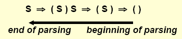
The right sentential form are the rightmost derivations of a string, and a parse of a string eats tokens left to right to reverse the rightmost derivation. A handle is a string defined by the expansion of a non-terminal in right sentential form.
Bottom-up parsing works by starting with an empty stack and having two operations: shift, putting the next input token onto the stack; and reduce, replacing the right-hand side of a grammar rule with its left-hand side. We augment the start state S with a rule Z → S (some books refer to this as S′ → S), making Z our new start symbol, so when only Z is on the stack and the input is empty, we accept. The parse stack is maintained where tokens are shifted onto it until we have a handle on top of the stack, whereupon we shall reduce it by reversing the expansion.
In this process, we can observe that when a rightmost non-terminal is expanded, the terminal to the right of it is in its Follow set - we need this information later on, and is also important to note that the Follow set can include $.
At any moment, a right sentential form is split between the stack and the input; each reduce action produces the next right sentential form. Given A → α, α is reduced to A if the stack content is a viable prefix of the right sentential form. Appropriate handles are at the base of the expansion triangles in the following right sentential form.
LR(0)
An LR(0) item is a way of monitoring progress towards a handle. It is represented by a production rule together with a dot. The right-hand side has part behind the dot and part in front. This says that the parse has matched a substring derivable by the component to the left of the dot and is now prepared to match something on the input stream defined by that component to the right of the dot, e.g.,
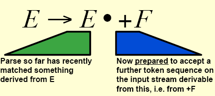
A production rule can therefore give rise to several configuration items, with the dots in varying places. When the dot is to the extreme left, we call this an initial item, and when the dot is to the extreme right, we call this a completed item, and these are typically underlined.
To represent the state and the progress of the parse, we can use a finite state automata. Typically, we start by construction a NDFA where each state of the NDFA contains an LR(0) item and transitions occur based on terminals and non-terminals. We then apply subset construction to obtain a DFA.
![]()
To traverse our newly constructed DFA, the stack now contains both symbols and DFA states in pairs. We can then use the algorithm described on slide 15 of lecture set 6. As LR(0) has no look-ahead, we can encounter problems with ambiguous grammars. If a state contains a complete item A → α. and another item A → α.Xβ, then there is a shift-reduce conflict. If a state contains a complete item A → α. and another complete item B → β., then there is a reduce-reduce conflict.
We say that a grammer is LR(0) if none of the above conflicts arise, that is, if a state contains a complete item, then it can contain no other item.
Another way of saying that a grammar is LR(0) is if its LR(0) parser is unambiguous. The LR(0) parsing table is the DFA and the LR(0) parsing actions combined.
LR(0) parsing belongs to a more general class of parsers, called LR parsers. NDFAs are built to describe parsing in progressively increasing levels of detail (similar to recursive descent parsing). The DFA, built from subset construction, builds the parse tree in a bottom-up fashion and waits for a complete right-hand side with several right-hand sides sharing a prefix considered in parallel. A stack is used to store partial right-hand sides (the handles) and remember visited states. The right-hand side is traced following arrows (going from left-hand side to right-hand side), and then removed from the stack (going against the arrows). The uncovered state and left-hand side non-terminal then define the new state.
LR parsers can also take advantage of a look-ahead symbols, similar as in top-down parsing where the left-hand side is expanded into the right-hand side based on a single look-ahead symbol (if any). The main LR parsing methods are:
- LR(0) - discussed above, uses no look-ahead
- SLR(1) - the left-hand side is only replaced with the right-hand side if the look-ahead symbol is in the Follow set of the left-hand side
- LR(1) - this uses a subset of the Follow set of the left-hand side that takes into account context (the tree to the above and left of the left-hand side)
- LALR(1) - this reduces the number of states compared to LR(1), and (if lucky), uses a proper subset of the Follow set of the left-hand side
SLR(1)
SLR(1) parsing works on the principle of look-ahead before shift and see what follows before reduce. The algorithm is described on slide 18 of lecture set 6.
We say that a grammar is SLR(1) if and only if:
- for any item A → α.Xβ where X is a terminal, there is no complete item B → γ. in the same state for which X ∈ Follow(B) - this avoids shift-reduce conflicts
- for any two complete items A → α. and B → β. in the same state, Follow(A) ∩ Follow(B) = ∅ - this avoids reduce-reduce conflicts
We can accomplish this by using some disambiguating rules, prefering shift over reduce solves the shift-reduce conflict (and as a direct implication, this implements the most closely nested rule). For reduce-reduce conflicts, the rule with the longer right-hand side is preferred.
LR(1)
Canoncical LR(1) parsing is done using a DFA based on LR(1) items. This is a powerful general parser, but is very complex, with up to 10 times more states than the LR(0) parser.
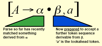
We can construct a LR(1) parser in the same way as a LR(0) parser, using the LR(1) items as nodes. However, the transitions are slightly different. For any X (terminal or non-terminal) the lookahead does not change:
![]()
We also have ε-transitions for every production B → β and for every token bi ∈ First(γa), where B is a nonterminal. This also changes the look-ahead symbol, unless γ → ε or γ = ε.
![]()
The LR(1) parsing table is the same format as for SLR(1) parsing, and the parsing algorithm is as described on slide 27 of lecture set 6.
We say that a grammar is LR(1) if and only if:
- for any item [A → α.Xβ, a], where X is a terminal, there is no complete item [B → α., X] in the same state - this removes shift-reduce conflicts
- there are no two complete items [A → α., a] and [B → β., a] in the same state
LALR(1)
The class of languages that LALR(1) can parse is between that of LR(1) and SLR(1), and in reality is enough to implement most of the languages available today. It uses a DFA based on LR(0) items and sets of look-aheads which are often proper subsets of the Follow sets allowed by the SLR(1) parser. The LALR(1) parsing tables are often more compact than the LR(1) ones.
We define the core of a state in an LR(1) DFA as the set of all LR(1) items reduced to LR(0) by dropping the lookahead.
As the LR(1) DFA is too complex, we can reduce the size by merging states with the same core and then extend each LR(0) item with a list of lookahead tokens coming from the LR(1) items of each of the merged states. We can observe that if s1 and s2 have the same core, and there is a transition s1 → t1 on symbol X, then there is a transition s2 → t2 on X, and t1 and t2 have the same core.
This gives us a LALR(1) parser, which is still better than SLR(1).
The LALR(1) algorithm is the same as the LR(1) algorithm, and an LALR(1) grammar leads to unambiguous LALR(1) parsing. If the grammar is at least LR(1), then the LALR(1) parser can not contain any shift-reduce conflicts. The LALR(1) parser could be less efficient than the LR(1) parser, however - as it makes additional reductions before throwing error.
Another technique to construct the LALR(1) DFA using the LR(0) DFA instead of the LR(1) DFA is known as propagating lookaheads.
Error Recovery
Similarly to LL(1) parsers, there are three possible actions for error recovery:
- pop a state from the stack
- pop tokens from the input until a good one is seen (for which the parse can continue)
- push a new state onto the stack
A good method is to pop states from the stack until a nonempty Goto entry is found, then, if there is a Goto state that matches the input, go - if there is a choice, prefer shift to reduce, and out of many reductions, choose the most specific one. Otherwise, scan the input until at least one of the Goto states like the token or the input is empty.
This could lead to infinite loops, however. To avoid loops, we can only allow shift actions from a Goto state, or, if a reduce action Rx is applied, set a flag and store the following sequence of states produced purely by reduction. If a loop occurs (that is, Rx is produced again), states are popped from the stack until the first occurence of Rx is removed, and a shift action immediately resets the flag.
The method Yacc uses for error recovery is NTi → error. The Goto entries of NTi will then be used for error recovery. In case of an error, states are popped from the stack until one of NTi is seen. error is then added to the input as its first token, and you continue going as if nothing has happened (you can alternatively choose to discard the original lookahead symbol). All erroneuous input tokens are discarded without producing error messages until a sequence of 3 tokens is shifted legally onto the stack.