What is AI?
There are many different competing definitions for AI, each with strengths and weaknesses. Some of them follow:
- AI is concerned with creating intelligent computer systems - however, we don't have a good definition of intelligent
- "AI is the study of systems that would act in a way that to any observer would appear intelligent" (Coppin) - this is dependent on the observer, and some observers that work in marketing have a very loose definition of intelligence.
We can define two types of AI from the above defintion:
- Weak AI - Machines can possibly act as if they were intelligent
- Strong AI - Machines can actually think intelligently
Alan Turing developed the Turing Test to check intelligence using the weak AI definition. The Turing Test is stuch that an interrogator is communicating with another group of people and a computer - however, he doesn't know which one. If 30% of the time (an arbitrary figure), the computers are able to fool the interrogator it is a real person, then the system has passed the Turing test.
Strong AI proponents have put forward the Chinese room test. A person P1 communicates in Chinese with another person, P2, by passing written notes back and forth. P2 does not know Chinese, however. P2 has a room full of books that tell him what to do for each character in the note (similar to a Turing machine). Assuming all the rules are correct, does P2 speak Chinese?
Other questions can be asked of intelligence. Goedel/Turing said that there are problems that computers are not able to compute (e.g., the halting problem), however the question must be asked - can humans? Therefore, are Turing machines the most powerful computational model?
Further definitions of AI include:
- "AI involves using methods based on intelligent behaviour of humans (or animals) to solve complex problems" (Coppin). This is nature orriented AI.
- AI is concerned with making computers more useful and useable - this definition is very vague, so it can be applied to all AI projects, but also to more general CS problems, and indeed could be the basis for all CS.
- AI is what AI researchers do - this is probably the best definition to date
Agents
"An agent is anything that can be viewed as perceiving its environment through sensors and acting upon that environment through actuators." (Russel and Norvig)
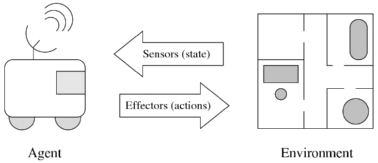
However, thermostats (which respond to changes in temperature by turning heating on or off) could also be included in that definition, but is not an AI.
Agents used to act only in closed systems, where the environment was very constrained and controlled, but now they are behaving in increasingly open environments.
We should consider intelligent agents, which can be defined by three characteristics according to Wooldridge (1999):
- Reactivity - Agents are able to perceive the environment and respond in a timely fashion to changes
- Proactiveness - Agents are able to exhibit goal-directed behaviour by taking initiative
- Social Ability - Agents are capable of interacting with other agents (and possibly humans)
This definition still includes thermostats, so it still has weaknesses.
Intelligent agents consist of various components which map sensors to actuators. The most important component is that of reasoning, which consists of representations of the environment (more than just pixels from a camera, but a semantic model which is a representation of the images), formulating a course of action (planning), path finding and steering, learning, social reasoning (competing and cooperating) and dealing with uncertainty (where the effects of an action are not known, so a decision must be made based on this).
Learning is very important, and there is a school of thought that all intelligent agents must learn. Learning can be broken up into supervised learning, where a teacher gives agent examples of things (sometimes called inductive learning), reinforcement learning, where the agent receives feedback of whether its behaviour is good or bad and learns from that (the carrot and stick approach) and unsupervised learning, which is the most difficult to implement, where the agent is given some basic concepts and then discovers things based on them (e.g., give a number system and let it discover prime numbers).
Another component of intelligent agents is perception, which is vision and language understanding, and the final component is acting, which is motion control and balancing.
Reasoning is done using search - looking at all possible ways and choosing the best one (e.g., path finding, learning, looking for the best action policy). Therefore, a possible definition of intelligent is whether or not the agent has done the right thing - a rational agent. The right thing here is defined by a performance measure - a means of calculating how well the agent has performed based on the sequence of percepts that it has received.
We can therefore define a rational agent such that for each possible percept sequence (complete history of anything the agent has ever perceived), a rational agent should select an action that is expected to maximise its performance measure, given the evidence provided by the percept sequence, and whatever built-in prior knowledge of the environment (knowledge that the agent designer has bestowed upon the agent before its introduction to the environment) the agent has.
Environments
There are different factors to consider when considering environments, such as:
- Fully vs. Partially Observable - the completeness of the information about the state of the environment
- Deterministic vs. Non-deterministic - Do actions have a single guaranteed effect (dependent on the state?)
- Episodic vs. Sequential - Is there a link between agent performance in different episodes?
- Static vs. Dynamic - Does the environment remain unchanged except by agent actions?
- Discrete vs. Continuous - is there a fixed finite number of actions and percepts?
- Single agent vs. Multi-agent
Programming AI
Two good languages for AI programming are Lisp, as programs can be treated as data and Prolog, which uses declarative programming.
Imperative/procedural programs say what should be done and how, so computation consists of doing what it says. Declarative/non-procedural programs say what needs to be done, but not how. Computation is performed by an interpreter that must decide how to perform the computation.
Logic programming is a form of declerative programming. Logic programs consist of statements of logic that say what is true of some domain. Computation is deduction; answers to queries are obtained by deducing the logical consequences of the logic program, thus, the interpreter is an inference engine. Programs can also contain information that helps guide the interpreter.
Problem Representation
A problem representation is defined by five items:
- set of states
- initial state
- finite set of operators - each is a function from states to states. The function may be partial as some operators may not be applicable to some states.
- goal test - can be explicit or implicit
- path cost - additive, so can be derived from the action costs
A solution is a sequence of operators that leads from the intial state to a state that satisfies the goal test.
Instead of operators, we could have successor functions. If s is a state then Successors is defined to be { x | x = op, for some operator op}
A problem representation can also be depicted as a state space - a graph in which each state is a node. If operator o maps state s1 to state s2, then the graph has a directed arc from s1 to s2 and the arc is labelled o. Labels could also be added to indicate the intial state and the goal states. Arcs can also be labelled to indicate operator costs.
Often a problem itself has a natural notion of configurations and actions. In such cases we can build a direct representation in which the state and operators correspond directly to the configurations and actions.
However, operators in the representation might not correspond directly to actions in the world. Some problems can be solved both ways, for example both towards and from the goal. If the real world has a natural direction, then we can refer to the search process as either forwards (if it matches the direction in the natural world) or backwards search.
An alternative view is that we can start with an empty sequence and fill in a middle state first, before filling in the first or last actions. In this view, states to not correspond directly to actions, but to the sequence built up so far - this is called indirect representation.
In direct representations, there is a close correspondence between problems and their representations, however it is important not to confuse them, especially because some representations are not direct. It is important to recognise that states are data structures (and they only reside inside a computer), and operators map data structures to data structures.
Search Trees
A problem representation implicitly defines a search tree. Root is a node containing the initial state. If a node contains s, then for each state s′ in Successors, the node has one child node containing the state s′. Each node in the search tree is called a search node. In practice, it can contain more than just a state, e.g., the path cost from the initial node. Search trees are not just state spaces, as two nodes in a tree can contain the same state.
Search trees could contain infinite paths, which we need to eliminate. This could be due to an infinite number of states, or where the state space contains a cycle. Search trees are always finitary (each node has a finite number of children), since a problem representation has a finite number of operators.
Search
As we saw earlier, given a problen representation, search is the process that builds some or all of the search tree for the representation in order to either identify one or more of the goals and the sequence of operators that produce each, or identify the least costly goal and the sequence of operators that produces it. Additionally, if the search tree is finite and does not contain a goal, then search should recognise this.
The basic idea of tree search is that it is an offline, simulated exploration of state space by generating successors of already-explored states (a.k.a., expanding states).
The general search algorithm follows the general idea that you maintain a list L containing the fringe nodes:
- set L to the list containing only the initial node of the problem representation
- while L is not empty do
- pick a node n from L
- if n is a goal node, stop and return it along with the path from the initial node to n
- otherwise remove n from L, expand n to generate its children and then add the children to L
- return Fail
Search is implemented where a state is a representation of a physical configuration, and a node is a data structure constituting part of a search tree that includes state, parent node, action, path cost, g(x) and depth.
Search algorithms differ by how they pick which node to expand. Uninformed search looks at only structure of the search tree, not at the states inside the nodes - this is often called blind search algorithms. Informed search algorithms make their decision by looking at the states inside the nodes - these are often called heuristic search algorithms.
Search algorithms can be evaluated with a series of criteria:
- Completeness - always finds a solution if one exists
- Time complexity - number of nodes generated (not expanded)
- Space complexity - maximum number of nodes in memory
- Optimality - always finds the least-cost solution
Time and space complexity are measured in terms of b - maximum branching factor in the search tree, d - depth of the least cost solution (root is depth 0) and m, the maximum depth of the state space (may be ∞)
Breadth First Search
See ADS.
BFS works by expanding the shallowest unexpanded node and is implemented using a FIFO queue.
It is complete, has a time complexity of Ο(bd + 1), space complexity of Ο(bd + 1) and is optimal is all operators have the same cost.
The space complexity is a problem, however, and additionally we can not find the optimal solution if operators have different costs.
Uniform Cost Search
This works by expanding the least-cost unexapanded node and is implemented using a queue ordered by increasing path cost. If all the step costs are equal, this is equivalent to BFS.
It is complete if the step cost ≥ ε, has a time complexity where the number of nodes with g ≤ the cost of the optimal solution, Ο(bceil(C*/ε)), where C* is the cost of the optimal solution, or Ο(bd). The space complexity is where the number of nodes with g ≤ cost of the optimal solution Ο(bceil(C*/ε)), or Ο(bd). This is optimal since nodes are expanded in an increasing order of g(n).
This still uses a lot of memory, however.
Depth First Search
This works by expanding the deepest unexpanded node, and is implemented using a stack/LIFO queue.
It is not complete, as it could run forever without ever finding a solution is the tree has an infinite depth. It does complete in finite spaces, however. The time complexity is Ο(bm), which is terrible if m >> d, but if solutions are dense, this may be faster than BFS. The space complexity if Ο(bm), i.e., linear space. It is not optimal.
Depth Limited Search
Depth limited search is DFS with depth limit l. That is, nodes deeper than l will not be expanded.
This solution is not complete, as a solution will only be found if d > l. It has a time complexity Ο(bl) and a space complexity Ο(bl). Also, the solution is not optimal.
Iterative Deepening Search
Depth limited search can be made complete using iterative deepening. The implementation of this is:
set l = 0
do
depth limited search with limit l
l++
until solution found or no nodes at depth l have children
This does have a lot of repetition of the nodes at the top of the search tree, so it's a class memory vs. CPU trade-off - this is CPU intensive, but only linear in memory. However, with a large b, the overhead is not too great, for example, when b = 10 and d = 5 the overhead is 11%.
IDS is complete, has a time complexity of (d + 1)b0 + db1 + (d - 1)b2 + ... + bd, or Ο(bd) and a space complexity of Ο(bd). Like BFS, it is optimal if step cost = 1.
Handling Repeated States
Failure to detect repeated states can turn a linear space into an exponential one. Any cycles in a state space will always produce an infinite search tree.
Sometimes, repeated states can be reduced or eliminated by changing the problem representation, e.g., by adding a precondition saying that the inverse of the previous operation is not allowed will eliminate cycles of length 2.
Another way of handing repeated states is by checking whether or not a node is equal to one of its ancestors, and don't add it if it is. For DFS-type algorithms, this is relatively easy to implement as all ancestors are already on the node list, however for other algorithms, this takes Ο(d) to traverse up the node list, or keeping a record of all the ancestors of a node, which consumes a lot of space.
A better way to solve this is to use graph search, which keeps track of all generated states. When a node is removed from the node list (the open list), it is stored on another list (the closed list). The basic version is the same as tree search, but you don't expand a node if it has the same state as one on the closed list. A more sophisticated version is required to retain optimality: If the new node is "cheaper" than its duplicate on the closed list, then the one on the closed list and its descendants must be deleted.
Siblings can still be created, however, so another way would be compare the node to all nodes - this is very expensive, so the normal solution to repeated states is to rewrite the problem representation.
We can consider the search algorithms above to be uninformed, that is, only the structure of the search tree and not at the states inside the nodes - these are blind search algorithms. We can improve these search algorithms by inspecting the contents of a node to see whether or not they are a good node to expand, we can call these type of algorithms informed search. The way of choosing whether or not a node is good is done using a heuristic, which makes a guess, using rules of thumb, as to whether that state is a good one or not. As these problems are NP-complete, heuristics are never accurate, but the guesses they make could be good.
The general search algorithm for informed search is called best-first search, although this is a slight misnomer, as if it were truly best-first, we would be able to go straight to the goal state. The general idea here is to use an evaluation function ƒ(n) for each node n, which gives us an estimate of desirability - only part of the evaluation functions needs to be a heuristic for the search to become informed. We then expand the most desirable unexpanded node. This is done by ordering the nodes in L in decreasing order of desirability, and nodes are always chosen from the front of L.
Greedy Best-First Search
In Greedy Best-First Search, the evaluation function ƒ(n) = h(n), our heuristic (an estimate of cost from n to the nearest goal). In our distance-finding example, this could be the straight line distance. Greedy Best-First Search therefore works by expanding the node that appears to be closest to the goal.
Greedy Best-First Search is not complete, as there a variety of cases where completeness is lost, e.g., it can get stuck in loops. The time complexity is Ο(bm), but a good heuristic can give dramatic improvement. The space complexity is also Ο(bm), as all nodes are kept in memory. Greedy best-first search is also not optimal.
A* Search
Greedy Best-First Search ignores the cost to get to the goal, which loses optimality. We therefore need to consider the cost to get to the node we are at. The basic idea of this is to avoid expanding paths that are already expensive. For this, we update our evaluation function to be ƒ(n) = g(n) + h(n), where g(n) is the cost so far to reach the node n - this is the same as uniform-cost search, therefore we can consider A* search to be a mixture of uniform-cost and greedy best-first search.
Even though the goal may be expanded by a previous expansion, it is never actually considered until it reaches the front of the list, as a more optimal path to the goal may be expanded from a node with a lower current cost.
A* search is sometimes referred to as A-search, however A* does have extra conditions for optimality compared to A. In A*, h(n) must be admissible, which guarantees optimality.
Using A* search, nodes are expanded in order of f value, which gradually adds so-called f-contours of nodes. A contour i has all nodes where f = fi, where fi < fi + 1.
A* is complete (unless there are infinitely many nodes with f ≤ ƒ(G) - as in uniform cost search). It also has a time complexity that is exponential in relative error in h and the length of the solution, and the space complexity is that of keeping all nodes in memory. It is also optimal.
Admissible Heuristics
A heuristic h(n) is admissible if ∀n h(n) ≤ h*(n), where h*(n) is the true cost to reach the nearest goal state from n, i.e., an admissible heuristic never overestimates the cost to reach the goal (i.e., it is optimistic).
For proof of optimality,
see lecture slides.
Theorem: If h(n) is admissible, A* using tree-search is optimal. That is, there is no goal node that has less cost than the first goal node that is found.
A heuristic is consistent if, for every node n, a successor n′ of n generated by any action a, h(n) ≤ c(n, a, n′) + h(n′), where c(n, a, n′) is the cost of getting from node n to n′ via action a. Using the triangle inequality (that is, the combined length of any two sides is always longer than the length of the remaining side), we have ƒ(n′) ≥ ƒ(n), i.e., ƒ(n) is non-decreasing along any path.
Theorem: If a heuristic is consistent, then it is admissible. The reverse is not strictly true, but it is very hard to come up with admissible heuristic that is not admissible.
Theorem: If h(n) is consistent, A* using graph-search is optimal. The proof for this is similar to that for uniform cost.
Admissible heuristics can be discovered by relaxing the problem to a simpler form (i.e., removing some constraints so it becomes easier to solve). If we have two heuristics where h1 is a relaxed form of h2 and both are admissible, then ∀n h2(n) ≥ h1(n), then we can say that h2 dominates h1.
Theorem: If h2 domaintes h1 then A* with h1 expands at least every node expanded by A* with h2.
Logic
Logic is the study of what follows from what, e.g., if two statements are true, then we can infer a third statement from it. It does not matter if the statements are actually true, just that if x and y is true, then z must also be true to be a valid statement.
Logic is useful for:
- Reasoning about combinatorial circuits
- Reasoning about databases
- Giving semantics to programming languages
- Formally specifying software and hardware systems - model-checking and theorem-proving can be used to show that the system meets the specification or that the system has certain properties.
- Capturing complexity classes (e.g., there is a correspondance between problems in NP and the forumlas of existential second-order logic - more precisely, a forumla and a problem correspond if there is a one-to-one mapping between the models satisfying the formula and the solutions to the problem)
- AIMA 7.6SAT (the satisfiability problem) solvers can solve practical problems. Cook showed all problems in NP can be polynomial reduced to SAT, but until recently no SAT solver could practically solve the very large number of clauses mapping an NP problem to SAT generates. Modern SAT solvers can now support up to 1,000,000 clauses so many practical problems can be solved by mapping them to SAT.
Logic is very important for AI as flexible, intelligent agents need to know facts about the world in which they operate - declerative knowledge and procedural knowledge - how to accomplish tasks. e.g., procedural - don't drink poison; declerative - drinking poison will kill you, and you want to stay alive.
Every way we can represent the world is a model, thus any model where the statement x is true, and y is true, we can infer a condition z based on those two statements. However, if we can infer a counter model where the premises are true, but the condition isn't, the argument is invalid.
Some words in an argument have set logical meanings, such as Some or Every, but others have variable meanings, such as foo or bar. Words that don't very in meaning are called logical symbols.
The semantics of a statement is whether or not a statement is true in a world, and is giving meaning to a statement.
Rule based systems use proof theory to take our arguments and check their validity, e.g., some X is a Y, every Y is a Z → some X is a Z is valid. We can express this as X/Y, Y/Z ∴ X/Z, which is valid and we don't need to consider the rules.
We need to consider a grammar, where we can express this formally, and the semantics that determine the validity of the arguments. Ways of doing this include propositional and first-order logic. The requirements for a declerative representation language are:
- The language should have syntax (a grammar defining the legal sentences)
- The language must have semantics (what must the world be like for a sentence to be true - truth-conditional semantics; there are other type of semantics dealing with other types of meaning, but we will not be dealing with that).
Intelligent agents need to reason with their knowledge, and many kinds of reasoning can be done with declarative statements:
- educated guesses
- reasoning by analogy
- jump to conclusions
- make generalisations
However, for LPA we will focus on sound, logical reasoning - i.e., deducing logical consequences of what is known, as determined by truth-conditional semantics.
Propositional Logic
As discussed above, we can discuss a declarative representation language using a syntax and a semantics. For propositional logic, our syntax consists of a lexicon and a grammar.
The lexicon (non-logical symbols) of propositional logic consists of a set of proposition symbols. Throughout the examples, we can assume that, P, Q, R, S and T are among the propositional symbols. The logical symbols of propositional logic are ¬, ∨, ^, →, ↔. We can then define the sentences of propositional logic as:
- If α is a proposition letter, then α is an atomic sentence
- If α and β are sentences, then (¬α), (α ∨ β), (α ^ β), (α → β) and (α ↔ β) are molecular sentences.
The above is an official definition, but we can take certain shortcuts to reduce clutter and to make writing logical statements easier. We can assign to connectives, from high to low, ¬, &or, ∧, →, ↔. We can then take advantage of this to omit paranthesis when no ambiguity results. Additionally, we can take the connectives ^ and ∨ to have an arbitary arity of two or more.
We call a sentence of the form α ∨ β a disjunction, where α and β are its disjuncts. A sentence of the form α ^ β is a conjunction, where α and β are its conjuncts.
We also need to consider the semantics of propositional logic. In propositional logic, a model is a function that maps every proposition letter to a truth value, either TRUE or FALSE. If α is a sentence, and I is a model, then [[α]]I is the semantic value of α relative to model I. [[α]]I is then defined as follows:
- If α is an atomic sentence, then [[α]]I = I(α)
- If α is (¬β) then [[α]]I = { TRUE if [[β]]I = FALSE, FALSE otherwise
- If α is (β ∨ γ) then [[α]]I = { TRUE if [[β]]I or [[γ]]I, FALSE otherwise
- If α is (β ^ γ) then [[α]]I = { TRUE if [[β]]I = TRUE and [[γ]]I = TRUE, FALSE otherwise
- If α is (β → γ) then [[α]]I = { TRUE if [[β]]I = FALSE or [[γ]]I = TRUE, FALSE otherwise
- If α is (β ↔ γ) then [[α]]I = { TRUE if [[β]]I = [[γ]]I, FALSE otherwise
An alternate way of thinking is if one thinks of the logical connectives as truth functions, which maps a pair of arguments to true or false in every model (which is why it is considered a logical symbol). Thus, we could define: [[(α ^ β)]]I = [[^]]([[α]]I, [[β]]I).
Theorem 1: Let A and A′ be two equivalent formulas. If B is a formula that contains A as a subformula, then B is logical equivalent to the formula that results from substituting A′ for A in B.
Theorem 2: Two sentences, A and B, are logically equivalent if and only if then sentence A ↔ B is valid.
Theorem 3: Let A, A1, ..., An be sentences. Then {A1, ..., An} entails A if and only if the sentence A1 ^ ... ^ An → A is valid.
An argument consists of a set of permises and another sentence called the conclusion. We allow the premises to be an infinite set. However, in many cases, we will be concerned with arguments that have a finite set of premises, and we can call these finite arguments. If an argument with premises P and conclusion C is valid, then we say that P entails C (or, C follows from P, or C is a consequence of P).
Let α be a sentence, A be a set of sentences and I be a model, then:
- I satisfies α if and only if [[α]]I = TRUE
- I satisfies A if and only if satisfies every a ∈ A
- I falsifies A if and only if [[α]]I = FALSE
- A (or α) is satisfiable if and only if it is satisfied by some model
- α is valid and unfalsifiable if and only if it is satisfied by every model
Note that although each individual sentence in A may be satisfiable, yet A itself may be unsatisfiable. For example, {P, ¬P} is unsatisfiable, yet P and ¬P are each satisfiable. Thus, not every unsatisfiable set of sentences if a set of unsatisfiable sentences. As we can see, the notion of a valid sentence is therefore different to the notion of a valid argument, but it is related.
There are some special definitions worth noting, however.
- The empty set of sentences if satisfied by every model, hence ∅ entail C if and only if C is a valid sentence
- An unsatisfiable sentences is entailed only by an unsatisfiable set of sentences
- A valid sentence is entailed by any set of sentences
Two sets of sentences are logically equivalent if they are satisfied by precisely the same models (they have the same truth value in all models). Two sentences are logically equivalent if and only if they entail each other.
First Order Predicate Calculus
Again, we start by considering the syntax of FOPC. The lexicon (non-logical symbols) of FOPC consist of the disjoint sets of a set of predicate symbols, each having a specified arity ≥ 0 (we often refer to symbols with arity 0 as proposition symbols - propositional logic is where all predicates have no arguments), and a set of function symbols, each having a specified arity ≥ 0 (function symbols of arity 0 are often called individual symbols, or often a a misnomer, constants), and finally a set of variables.
The logical symbols of FOPC consist of the quantifiers ∀ and ∃, and the logical connectives ¬, ^, ∨, → and ↔.
We can define the terms of FOPC as individual symbols, variables, and function symbols, where if ƒ is a function symbol of arity n and t1, ..., tn are terms then ƒ(t1, ..., tn) is a term.
The formulas of FOPC are defined as atomic formulas, where if P is a predicate symbol of arity n and t1, ..., tn are terms, then P(t1, ..., tn) is an atomic formula, and as molecular formulas, where if α and β are formulas, then ¬α, (α ∨ β), (α ^ β), (α → β) and (α ↔ β) are molecular formulas. Additionally, if x is a variable and α is a formula, then (∀xα) and (∃xα) are molecular formulas.
We can consider variables to be either bound or free. We say that a variable x occuring in a formula α is bound in α if it occurs within α as a subformula of the form ∀xβ or ∃xβ. Otherwise we call the variable free. We call a formula α a sentence if there is no free occurance of a variable.
Sentences have truth values, as FOPC is based on compositional semantics, where the total truth value is equal to the sum of its parts.
Like with propositional logic, we can drop paranthesis if no ambiguity results, and we often give connectives and quantifiers precedence from high to low (¬, ∨, ^, →, ↔, ∀, ∃). We often specifiy ∀x1, x2, ..., xn as a shorthand for ∀x1, ∀x2, ..., ∀xn, and similarly for ∃.
If a term or formula contains no variables, we refer to it as ground. α ∨ β is a disjunction, where α and β are its disjuncts and α ^ β is a conjunction, where α and β are its conjuncts.
We can also consider first order propositional logic, which is first order predicate calculus with equality. The equality symbol "=" is both a logical symbol and a binary predicate symbol. Atomic formulas using this predicate symbol are usually written as (t1 = t2), instead of =(t1, t2). Also, we usually write (t1 ≠ t2) instead of ¬(t1 = t2).
To consider the semantics of FOPC, we define a pair (D, A), where D is a potentially infinite non-empty set of individuals called the domain and A is a function that maps each n-ary function symbol to a function from Dn to D and each n-ary predicate symbol to a function Dn to {TRUE, FALSE}. Individual symbols (function symbols of 0-arity) always map to an element of D and a predicate symbol of arity 0 (i.e., a proposition symbol) is mapped to TRUE or FALSE.
When we are considering formula with free variables, the truth value depends not only on what model we are considering, but what values we give to these variables. For this purpose, we will consider the value of an expression relative to a model and a function from variables to D. Such a function is called a value assignment.
For a full semantic
definition of all symbols
see lecture notes.
If α is an expression or a symbol of the language, then [[α]]I, gis the semantic value of α relative to model I and value assignment g. If g is a value assignment, then g[x ↵ i] is the same value assignment, with the possible exception that g[x → i](x) = i.
Proof Systems
Proof systems work by a syntactic characterisation of valid arguments. Here, we will consider the Hilbert, or axiomatic, system. These systems work by starting with the set of premises of the argument, and repeatedly apply inference rules to members of the set to derive new sentences that are added to the set, the goal being to derive the conclusion of the argument. Some proof systems start with a possibly infinite set of logical axioms (e.g., every sentence of the form α ^ ¬α).
Propositional Logic
Many proof systems for propositional logic employ a wide variety of rules. Commonly used rules include and-introduction - from any two sentences α and β, derive α ^ β - and modus ponens - from any two sentences of the form α and α → β, derive β.
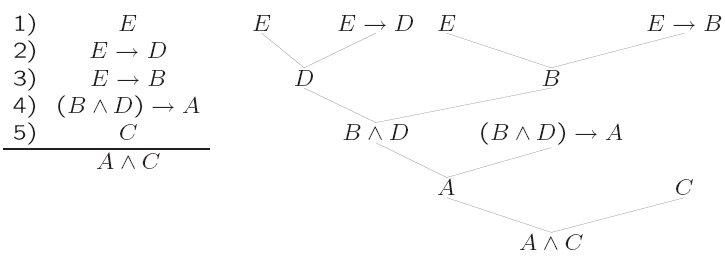
If we consider the following argument, we can show that the conclusion is derived from the premises:
A
A → B
A → C
Then we can derive the result as follows:
- A - premise
- A → B - premise
- A → C - premise
- B - modus ponens from 1 and 2
- C - modus ponens from 1 and 3
- B ^ C - and-introduction from 4 and 5
Derivations can also be represented as trees and as directed, acyclic graphs, e.g.,
We can say a proof system is sound if every sentence that can be derived from a set of premises is entailed by the premises, and that a proof system is complete if every sentence that is entailed by a set of premises can be derived from the set of premises. Therefore, we can consider soundness and completeness when the set of sentences derivable from a set of premises is identical to the set of sentences entailed by the premises. This is obviously a desirable property.
An inference rule of the form: From α1, ..., αn derive β, is sound if {α1, ..., αn} entails β. Modus ponens and and-introduction are sound.
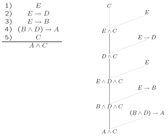
Some proofs are linear, that is when the shape of their tree looks as follows:
We can also reason backwards, where a proof can be turned upside down and we start from the conclusion and work towards [], the truth condition.
Horn Clauses
Each premise in a propositional Horn clause argument is a definite clause (α1 ^ ... ^ αn) → β, where n ≥ 0 and each αi and β is atomic. If n = 0, then we have that → β is a definite clause, and we usually write this as simply β.
The conclusion in a propositional Horn clause argument is a conjunction of atoms α1 ^ ... ^ αn. As a special case, we can consider [] when n = 0. We call this the empty conjunction and it is true in all models.
SLD Resolution for Propositional Logic
The SLD resolution inference rule is used to derive a goal clause from a goal clause and definite clause.
From the goal clause G1 ^ ... ^ Gi - 1 ^ Gi ^ Gi + 1 ^ ... ^ Gn (n ≥ 1) and the definite clause B1 ^ ... ^ Bm → H (m ≥ 0) we can derive the goal clause G1 ^ ... ^ Gi - 1 ^ B1 ^ ... ^ Bm ^ Gi + 1 ^ ... ^ Gn, provided that H and Gi are identical.
Because of their special form, SLD proofs are often shown simply as:
A ^ C
B ^ D ^ C (4)
E ^ D ^ C (3)
E ^ C (2)
C (1)
[] (5)
Where the number following is the number of the premise that SLD resolution was applied to.
The element of the goal clause that is chosen to have SLD resolution applied to it is chosen using a selection function, and the most common selection functions are the leftmost and rightmost selection functions.
We have the following properties about SLD inference:
- The SLD inference rule is sound and complete for propositional Horn-clause arguments
- Selection function independence - Let S1 and S2 be selection functions and let A be a Horn-clause argument. Then, there is an SLD resolution proof for A that uses S1 if and only if there is one that uses S2.
SLD Resolution for First Order Predicate Calculus
The goal here is to generalise SLD resolution for propositional Horn-clause arguments to handle first order Horn-clause arguments (i.e., a subset of predicate calculus).
If we let Φ be a forumla whose free (unbound) variables are x1, ..., xn, then Φ is the universal closure of Φ, which abbreviates ∀x1, ..., xn Φ. Furthermore, Φ is the existential closure of Φ and abbreviates ∃x1, ..., xn Φ.
Each premise in a first order Horn-clause argument is a definite clause((α1 ^ ... ^ αn) → β), where n ≥ 0 and where each αi and β are atomic formulas of first order predicate calculus. If n = 0, then we have that (→ β), which is a definite clause and we simply write this as β.
The conclusion in a propositional Horn-clause argument is a goal clause (α1 ^ ... ^ αn), where each αi is an atomic formula of first-order predicate calculus. As a special case when n = 0, we can write [] - this is the empty conjunction which is true in all models.
Since all variables in the definite clause are univerally quantified, and all those in the goal clause are existentially quantified, the closures are often not written, so in such cases, it is important to bear in mind that they are there implicitly.
Substitutions
A substitution is a function that maps every expression to an expression by replacing variables with expressions whilst leaving everything else alone. Application of a substitution θ to an expression e is written as eθ rather than θ(e). We only need to consider applying substitutions to expressions containing no quantifiers to simplify the presentation.
A more formal definition of a substitution is that: A substitution is a function θ from expressions to expressions such that for every expression e: if e is a constant then eθ = e. If e is composed of e1, e2, ..., en then eθ is composed of e1θ, e2θ, ..., enθ in the same manner. If e is a variable, then eθ is an expression.
We can consider the identity function as a substitution, usually called the identity substitution. We can observe that substitutions are uniquely determined by their treatment of the variables; that is θ1 = θ2 if and only if vθ1 = vθ2 for every variable v.
The domain of a substitution is the set containing every variable that the substitution does not map to itself. The domain of the identity substitution is the empty set.
An algorithm needs a systematic way of naming each substitution it uses with a finite expression. Since we are only concerned with substitutions with finite domains, that can be accomplished straightforwardly.
Suppose that the domain of a substitution θ is {x1, ..., xn} and that each xi is mapped to some expression ti, then θ is named by {x1 → t1, ..., xn → tn}. The empty set names the identity substitution and {x → y, y → x} names the substitutions that swaps xs and ys throughout an expression.
Instances
An expression e′ is said to be an instance of expression e if and only if e′ = eθ for some substitution θ (i.e., eθ is an instance of e).
As the identity function is a substitution, we could say that every expression is an instance of itself.
An expression is ground if and only if it contains no variables. We shall be especially concerned with the ground instances of an expression, which obviously are the instances of the expression which contains no variables.
We can write egr to denote the set of all ground instances of the expression e. By extension, if E is a set of expressions, then Egr denotes the set of all ground instances of all expressions in E, that is Egr = ∪e ∈ E egr.
Herbrand's Theorem
Herbrand's Theorem is that by considering ground instances, we can relate the validity of first order Horn clause arguments to those of propositional logic. This relationship offers us guidance on how to generalise the SLD resolution inference rule from propositional logic to first order predicate calculus.
The theorem is: "Let P be a set of definite clauses and G be a goal clause. Then, P entails G if and only if Pgr entails some ground instance of G."
The Herbrand theorem gives us an idea of how SLD resolution should work for first order Horn clause arguments. The best way to demonstrate this is with some example arguments and their SLD search spaces.
(1) P(a)
(2) P(c) → P(d)
(3) R(d) → P(e)
(4) R(d)
P(x)
(1) [] - considering x replaced by a
(2) P(c) - considering x replaced by d
(3) R(d) - considering x replaced by e
(4) []
Where variables occur in the premises, they can be replaced by any constant in a similar way to variables in the goal, as long as the variable replacements are consistent.
Unifiers
A substitution θ is said to unify expressions e1 and e2 if e1θ = e2θ. We call these two expressions unifiable, and θ is the unifier. The set of the set of all unifiers of two expressions can be characterised by a greatest element, the most-general unifier.
If we let e1 and e2 be two expressions that have no variables in common, then e1 and e2 are unifiable if and only if the intersection of (e1)gr and (e2)gr is non-empty. Furthermore, if they are unifiable and θ is their most general unifier, then (e1θ)gr = (e2θ)gr = (e1)gr ∩ (e2)gr.
We can say that a substitution θ solves an equation e1 = e2 if e1θ= e2θ. We say that a substitution solves a set of equations if it solves every equation in the set. (Note that ∅ is solved by every substitution). Thus, we can view the problem of finding a most general unifier of e1 and e2 as that of finding the most general solution to e1 = e2. The unification algorithm finds a most general solution to any given finite set of equations by rewriting the set until it is in such a form that a most general solution to it is readily seen.
An occurance of an equation in an equation set is in solved form if the equation is of the form x = t and x does not occur in t or in any other equation in the equation set. A set of equations is in solved form if every equation in the set is in solved form. {x1 → t1, ..., xn → tn} is a most general solution to the solved form set of equations {x1 = t1, ..., xn = tn}.
The unification algorithm takes two expressions, s1 and s2, and outputs either a substitution or failure. We let X be the singleton set of equations {s1 and s2} and repeatedly perform any of the four unification transformations until no transformation will apply. The output is of the form {x1 → t1, ..., xn → tn}, where x1 = t1, ..., xn = tn are the equations that remain in X.
The four unification transactions are:
- Select any equation of the form t = x, where t is not a variable and x is a variable, and rewrite this as x = t
- Select any equation of the form x = x, where x is a variable and erase it
- Select any equation of the form t = t′ where neither t nor t′ is a variable. If t and t′ are atomic and identical, then erase the equation, else if t is of the form ƒ(e1, ..., en) and t′ is of the form ƒ(e′1, ..., e′n), then replace t = t′ by e1 = e′1, ..., en = e′n, else fail.
- Select any equation of the form x = t where x is a variable that occurs somewhere else in the set of equations and where t ≠ x. If x occurs in t, then fail. Else, apply the substitution {x → t} to all other equations (without erasing x = t).
The unification algorithm is correct by the theorem that: the unification algorithm performs only a finite number of transformations on any finite input; if the unification algorithm returns fail, then the initial set of equations has no solutions; if the unification algorithm returns a set of equations then that set is in solved form and has the same solutions as the input set of equations.
With this, we can apply SLD-resolution for first order Horn clause arguments. From the goal clause G1 ^ ... ^ Gi - 1 ^ Gi ^ Gi + 1 ^ ... ^ Gn (n ≥ 1) and the definite clause B1 ^ ... ^ Bm → H (m ≥ 0) we can derive the goal clause (G1 ^ ... ^ Gi - 1 ^ B1 ^ ... ^ Bm ^ Gi + 1 ^ ... ^ Gn)θ, provided that H and Gi are unifiable and θ is the most general unifier of the two.
The SLD-resolution inference rule is sound and complete for first-order Horn clause arguments, and selection function independence also applies in the first-order case.
Answer Extraction
Definite clauses are so-named because they do not allow the expression of indefinite (disjunctive) information. e.g., given the premises thief(smith) ∨ thief(jones) and the conclusion ∃x thief(x), the conclusion follows, but we can not name the thief. This situation would never arise if the premises were definite clauses.
If we let P be a set of definite clauses and let C be a formula without any quantifiers, then P entailsC if and only if P entails some ground instance of C. If Cθ is a ground instance that is entailed, then θ is said to be an answer.
We know that if a first-order Horn clause argument is valid then it has an SLD proof, and it is easy to extract an answer from the proof. Furthermore, if we consider all SLD proofs for an argument, then we can extract all answers.
Answers are extracted by attaching to each node in the search space an answer box that records the substitutions made for each variable in the goal clause. The answers are then located in the answer box attached to each empty clause in the search space.
Constraint Satisfaction
An instance of the finite-domain constraint satisfaction problem consists of a finite set of variables X1, ..., Xn, and for each variable Xi a finite set of values, Di, called the domain (although Russel and Norvig require this to be non-empty, common practice is to allow empty domains, as they are useful), and a finite set of constraints, each restricting the values that the variables can simultaneously take.
A total assignment of a CSP maps each variable to an element in its domain (it is a total function), and a solution to the CSP is a total assignment that satisfies all the constraints.
Once you have an instance of a CSP, the goal is usually to find whether the instance has any solutions (satisfiable), to find any or all solutions, or to find a solution that is optimal for some given objective function (combinatorial optimisation).
Constraints in a CSP have an arity, the number of variables it constrains - constraints of arity 2 are referred to as binary constraints.
The satisfiability problem for a CSP is NP-complete, and this can be proven by reducing CSP to SAT, where the variables are proposition letters, domains are True or False and the constraint is that the entire thing must evaluate to True. Therefore, no polynomial algorithm is going to work, and we need to search in some form.
Here, we are only looking at constraint satisfaction for discrete, finite domains. Other constraint satisfaction problems (other the domain of reals) include linear programming (in polynomial time), non-linear programming and integer linear programming (NP-complete). Other extensions to the basic problem include soft constraints, dynamic constraints and probabilistic constraints.
Constraints are expressed extensionally, where a constraint among n variables is considered as a set of n tuples. IfX1, ..., Xn are variables with domains D1, ..., Dn, then a constraint among these variables is a subset of D1 × ... × Dn. The traditional way, especially for theoretical studies, abstracts away from any language for expressing constraints, although it can be thought of as a disjunctive normal form.
In a constraint language, we can use operators such as = (equality),≠ (disequality), inequality on domains with an ordering (< or >), operators on values or variables, such as + or ×, logical operators such as ocnjunction, negation and disjunction, and constraints and operators specific to particular domains, such as alldifferent(x1, ..., xn) or operations on lists, intervals and sets.
CSP solving is often effective in many cases, and can be solved by first modelling, where a problem is formulated as a finite CSP (similar to reducing the problem), solving the CSP (there is powerful technology available to solve even large instances of a CSP that arise from modelling important real-world problems) and then mapping the solution to the CSP to a solution to the original problem.
CSP solving methods include constraint synthesis, problem reduction or simplification, total assignment search (also called local search or repair methods, e.g., hill-climbing, simulated annealing, genetic algorithms, tabu search or stochastic local search), and partial assignment search (also called constraint satisfaction search, partial-instantiate-and-prune and constraint programming). Searches can be classified by two criteria: stochastic or non-stochastic and systematic or non-systematic search.
Partial Assignment Search
To find a solution by partial assignment search, a space of partial assignments is searched, looking for a goal state which is a total assignment that satisfies all the constraints.
In partial assignment search, you start at the initial state with an assignment to no variables. Operators are then applied, each of which extends the assignment to cover an additional variable. Some reasoning is then performed at each node to simplify the problem and to prune nodes that can not extend to reach a solution.
Partial assignment uses a method called backtrack. If all the variables of a constraint are assigned and the constraint is not satisfied then the node containing that constraint is pruned.
Partial assignment search for an instance I of the CSP can be shown as a problem representation:
- States: A state consists of a CSP instance and a partial assignment
- Initial State: The CSP instance I and the empty assignment. Problem reduction is often performed to simplify the initial state
- Goal States: Any state that has not been pruned and the assignment is total
- Operators: A variable selection function (heuristic) is used to choose an unassigned variable, Xi. Then, for every value v in the domain of Xi, there is an operator that produces a new state by:
- Extending the assignment by assigning v to Xi
- Setting D i to {v}
- Performing problem reduction to reduce the domains
- Pruning the new node if any domain is the empty set
- Path Cost: This is constant for each operator application
There are issues in partial assignment search, however - how do we know what problem reductions should be performed, how are variables selected, how the search space is searched and how the values are ordered.
Given a problem state (a set of variables with domains, a partial assignment to those variables and a set of constraints), then we should be able to transform it to a simpler, but equivalent problem state.
Sometimes the simplified problem state will be so simple that it may be obvious what the solutions are, or that there are no solutions. In the non obvious states search continues.
Other techniques for reduction include domain reduction.
Consistency Techniques
Consistency techniques are a class of reduction techniques that vary in how much reduction they achieve and how much time they take to compute. In the extreme, there are some consistency techniques that are so powerful that they solve a CSP by themselves, but these are too slow in practice. At the other extreme, one could also solve by search with little or no simplifcation, which is also ineffective.
For many applications, generalised arc consistency (GAC) provides an effective trade-off for a wide class of problems. Node consistency is a special case of GAC for unary constraints and arc consistency is a special case for binary constraints. Other consistency techniques could also be effective for specific problems.
Node Consistency
A unary constraint C on a variable x is node consistent if C(v) is true for every value v in the domain of x.
A CSP is node consistent if all of its unary constraints are node consistent.
To achieve node consistency on a constraint C(x), remove from the domain of x every value vx, such that C(vx) is false. Node consistency on a problem is achieved by achieving it once on each unary constraint.
If a CSP instance is node consistent, that all of its unary constraints can be removed without changing the solutions to the problem. Whether or not a CSP instance is satisfiable is independent of whether or not it is node consistent, as shown in the table below:
| odd(x) | Sat | Sat |
|---|---|---|
| NC | Dx = {1} | Dx = {} |
| NC | Dx = {1,2} | Dx = {2} |
Arc Consistency
This is the binary case of generallised arc consistency. A constraint C on variables x and y is arc consistent from x to y if and only if for every value vx in the domain of x there is a value vy in the domain of y such that {x → vx, y → vy} satisfies C. Alternatively we could say that every value in x takes part in some solution of C.
A constraint C between x and y is arc consistent (written AC(C)) if it is arc consistent from x to y and y to x.
An instance of a CSP is arc consistent if all of its constraints are arc consistent. Whether or not a CSP instance is satisfiable is independent of whether or not it is arc consistent:
| x ≠ y | Sat | Sat |
|---|---|---|
| AC | Dx = {1} Dy = {2} |
Dx = {} Dy = {} |
| AC | Dx = {1,2} |
Dx = {1} Dy = {1} |
Arc consistency is directional and is local to a single constraint.
If applying arc consistency to a constraint C results in x having an empty domain if and only if C is unsatisfiable. Applying arc consistency from x to y would also result in y having an empty domain if and only if x does.
Generalised Arc Consistency
A constraint C on a set {x0, x1, ..., xn} is generalised arc consistent from x0 if and only if for every value of v0 in the domain of x0 there are values v1, ..., vn in the domains of x1, ..., xn such that {x0 → v0, ..., xn → vn satisfies C. Alternatively, we could say that every value in the domain of x0 takes part in some solution of C.
A constraint C on a set X of variables is generalised arc consistent (written GAC(C)), if and only if it is generalised arc consistent from every x ∈ X. An instance of the CSP is generallised arc consistent if all of its constraints are generalised arc consistent.
This is a generalisation of both node and arc consistency. A binary constraint is arc consistent if and only if it is generalised arc consistent. A unary constraint is node consistent if and only if it is generalised arc consistent.
Domain Reduction during Search
There are three main techniques for applying domain reduction during search:
- Backtracking: When all variables of a constraint are assigned, then check if the constraint is satisfied - if not, then prune. This is almost always ineffective as it does not perform enough pruning.
- Forward Checking: When all variables are assigned, but one variable of a constraint C is assigned, then achieve generalised arc consistency from the unassigned variable to the other variables and prune if a domain becomes empty.
- Maintaining Arc Consistency: Achieve GAC at each node, and prune if a domain becomes empty.
Variable Ordering
Variable ordering can affect the size of the search space dramatically. There are two main techniques to variable ordering: static, which is satisfied before the search begins and is the same down every path; and dynamic, where the choice depends on the current state of the search, and hence can vary from path to path.
The most common type of variable ordering is based on the fail-first principle. A variable with the smallest domain is chosen, and ties can be broken by choosing a variable that participates in most constraints. This is static if no simplification is done and is dynamic if simplification reduces domain sizes. This method often works well and is built into many toolkits.
Other methods sometimes work better for particular problems, such as in laying out a PCB to place the largest components first, and in class timetabling to timetable the longest continuous sessions.
Once the variables have been ordered and a pruning method selected, we have a search space, however we need to consider how to search this space. Standard depth first search is used, however a variety of advanced methods for dependency-directed backtracking exist. Instead of backing up one level on failure, it can sometimes be inferred that there can be no solution unless search backs up several levels.
When choosing a value from the search space, we have to consider ordering them. This has no effect if no solution exists or all solutions are to be found. The first strategy is to arbitrarily choose a value - this is a popular strategy. Other strategies include, for each value, forward check and choose one that maximises the sum of the domain sizes of the remaining variables, and the final strategy is for each value, to forward check and choose one that maximises the product of the domain sizes of the remaining variables.
Particular problems may also have simple strategies that enable the choice of a value most likely to succeed.
Planning
A planner takes an initial state and a goal, and then uses a process known as planning to put the world into a state that satisfies the goal. Principally, there is no difference between this and search (as for most AI techniques). However, in a simple search (where all applicable actions are taken in a state, and then the resulting states are checked to see if they are a goal state), this becomes infeasible even in moderately complex domains. A solution to this problem is to exploit information about actions, so irrelevant actions are never chosen (e.g., for an AI driver, if your goal is to get from A to B, then you don't need to alter the air conditioning).
Situation Calculus
Situation calculus is one method of representing change in the world. Situation calculus works by maintaining an up-to-date version of the state of the world, by tracking changes within it. The language of situation calculus is first order logic.
Situation calculus consists of:
- domain predicates, which represent information about the state of the world
- actions
- atemporal axioms, which consist of general facts about the world
- intra-situational axioms, which are facts about situations
- causal axioms, which describe the effects of actions
Predicates that can change depending on the world state need an extra argument to say in what state they are true, e.g., in the blocks world, held(x) becomes held(x, s), etc... Predicates that do not change do not need the extra argument, e.g., block(x).
We also have a function called result(a, s), which is used to describe the situation that results from performing an action a in a situation s.
Causal axioms model what changes in a situation that results from executing some action, not what stays the same. Therefore, we need to define frame axioms which define what stay the same in a situation. This necessity causes the frame problem, as in a complex domain, a lot of things stay the same after an action has been executed.
Finding a sequence of actions that leads to a goal state can be formulated as an entailment problem in first order predicate calculus. For situation calculus planning, the steps to take are to specify an initial state (as state s0), specify a goal (a formula that contains one free variable S) and then find a situational term such that the goal is a logical consequence of the axioms and the initial state. A situation term is a ground term of nested result expression that denotes a state.
We can formally state this as: Given a set of axioms D, an initial state description I and a goal condition G, find a situation term t such that G {S → t} is a logical consequence of D ∪ I.
Situation calculus does have limitations, however - it has a high time complexity, does not support simultaneous actions, does not handle external actions, or other changes than those brought about as a direct result of the actions, it assumes that all actions are instantaneous, and there is no way to represent time.
As we can see, there are multiple problems with planning, such as the frame problem (both representational and inferential), the qualification problem (it is difficult to define all circumstances under which an action is guaranteed to work) and the ramification problem (there is a proliferation of implicit consequences of actions).
STRIPS
STRIPS is the Stanford Research Institute Problem Solver, and also the formal language that the problem solver uses. It provides a representation formalism for actions and has the idea that everything stays the same unless explicitly mentioned - this avoids the frame problem.
Again, STRIPS uses propositional or first order logic, and the state of the world is represented by a conjunction of literals. There is one restriction, and that is that first-order literals must be ground and function-free. STRIPS uses the closed world assumption, that is, everything that is not mentioned in a state is assumed to be false. In STRIPS, the goal is represented as a conjunction of positive (that is, non negated) literals. In the propositional case, the goal is satisfied if the state of the world contains all the propositional atoms. In the first-order case, the goal is satisfied if the state contains (all) positive literals in the goal.
The STRIPS representation consists of a state (a conjunction of function-free literals), a goal (a conjunction of positive function-free literals - they can however contain variables, which are assumed to be existentially qualified) and an action (represented by a set of pre-conditions that must hold before it can be executed and a set of post-conditions, i.e., effects that happen when it is executed). It is common practice to seperate the effects (post-conditions) of an action in STRIPS into an add list, which contains the positive literals, and a delete list which contain the negative literals, for the sake of readability.
An action is said to be applicable if in some state, the state satisfies the actions preconditions (i.e., all literals in the preconditions are part of the state). To establish applicability for first-order actions (action schemas), we need to find a substitution for the varibles that make the action applicable.
The results of an action are that the positive literals in the effect are added to the state, and any negative literals in the effect that match existing positive literals in the state make the positive literals disappear, with the exceptions of positive literals already in the state are not added again, and negative literals that match with nothing in the state are ignored.
Regression Planning
Planning in STRIPS can be seen as a search problem. We can move from one state of a problem to another in both a forward and backward direction because the actions are defined in terms of both preconditions and effects. We can use either forward search, called progression planning, or backward search, known as regression planning.
Forward planning is equivalent to forward search, and as such is very inefficient and suffers from all of the same problems as the underlying search mechanism. A better way to solve the planning problem is through backwards state-space search, i.e., starting at the goal and working our way back to the initial state. With backwards search, we need to only consider moves that achieve part of the goal, and with STRIPS, there is no problem in finding the predecessors of a state.
To do regression planning, all literals from the goal description are put into a current state S (the state to be achieved). A literal is then selected from S, and an action selected that contains the selected literal in its add list. The preconditions of the selected action are added to the current state S and literals in the add list are removed from S. When the start state is a subset of the current list of literals of S, we can return success.
Whilst doing regression planning, we must insist on consistency (i.e., that the actions we select do not undo any of the desired goal literals).
This state space search method is still inefficient however, so we should consider whether or not we can perform A* search with an admissible heuristic.
Subgoal Independence
It is often beneficial to assume that the goals that we have to solve do not interact. Then, the cost of solving a conjunction of goals is approximated to the sum of the costs of solving each individual goal seperately. This heuristic is:
- optimistic (and therefore admissible) when the goals do interact, i.e., an action in a sub plan deletes a goal achieved by another subplan
- pessimistic (inadmissible) when subplans contain redundant actions
Empty Delete List
This heuristic assumes that all actions have only positive effects. For example, if an action has the effects A and ¬B, the empty delete list heuristic considers the action as if it only had the effect A. In this way, we can assume that no action can delete the literals achieved by another action.
Sussman Anomaly
The Sussman Anomaly is a situation in the blocks world that can be solved effectively using the planning methods discussed above.
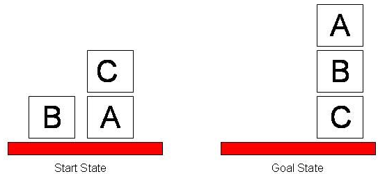
The initial state is On(C, A), Ontable(A), Ontable(B), Handempty and the goal state is On(A, B), On(B, C).
One way of solving this anomaly is to add the condition Ontable(C), however another way is to use another method of planning known as partial order planning.
Partial Order Planning
Up until now, plans have been totally ordered, i.e., the exact temporal relationships between the actions are known. In partially ordered plans, we don't have to specify the temporal relationships between all the actions, and in practice this means that we can identify actions that happen in any order.
Above, we have searched from the intial state to the goal or the vice versa. A complete plan is one which provides a path from the initial state to the goal, and a partial plan is one which is not complete, but could be extended to be complete by adding actions at the end (forwards) or at the beginning (backwards) of it. We then need to consider whether or not we can search this space of partial plans.
Doing planning as search happens in the space of partially ordered partial plans, where the nodes are the partially ordered partial plans. The edges denote refinements of the plans, i.e., adding a new action and constraining the temporal relationships between two actions. The root (initial) node is the empty plan, and a goal is a plan that, when executed, solves the original problem.
We represent a plan as a tuple (A, O, L) where:
- A is a set of actions
- O is a set of orderings on actions, e.g., A < B means that action A must take place before action B
- L is a set of causal links which represent dependencies between actions, e.g., (Aadd, Q, Aneed) means that Q is a precondition of Aneed and also an effect of Aadd. Obviously we still have to maintain that Aadd < Aneed.
We also need to consider threats - we say that an action threatens a causal link when it might delete the goal that the link satisfies. The consequences of adding an action that breaks a causal link into the plan are serious. We have to make sure to remove the threat by demotion (move earlier) or promotion (move later).
The partial order planning (POP) algorithm works as follows:
- Create two fake actions, start and finish
- start has no preconditions and its effects are the literals of the intial state
- finish has no effects and its preconditions are the literals of the goal state
- an agenda is created which contains pairs (precondition, action) and initially contains only the preconditions of the finish action
- while the agenda is not empty:
- select an item from the agenda (i.e., a pair (Q, Aneed))
- select an action Aadd whose effects include the selected precondition Q
- If Aadd is new, add it to the plan (i.e., to the set of actions A)
- Add the ordering Aadd < Aneed
- Add the causal link (Aadd, Q, Aneed)
- Update the agenda by adding all the pre-conditions of the new action (i.e., all the (Qi, Aadd)) and remove the previously selected agenda item
- Protect causal links by checking whether Aadd threatens any existing links, and check existing actions for threats towards the new causal links. Demotion and promotion can be used as necessary to remove threats
- Finish when there are no open precondition
Other Approaches to AI
The agents we have looked at above are known as logic-based agents, where an agent performs logic (symbolic) reasoning to choose the next action, based on percepts and internal axioms. Logic based agents have the advantages of the ability to use domain knowledge, and the behaviour of agents have clean logical semantics. However, logic reasoning takes times (sometimes a considerable amount of time), so the computed action may no longer be optimal at execution time (i.e., logic causes calculative rationality). Additionally, representing and reasoning about dynamic, complex environments in logic is difficult, and as logic-based agents operate on a set of symbols that represent entities in the world, mapping the percepts to these symbols is often difficult and problematic.
Reactive Agents
Reactive agents are baed on the physical grounding hypothesis and this is sometimes referred to as Nouvelle AI or situated activity (Brooks, 1990).
Here, intelligent systems necessarily have their interpretations grounded in the physical world, and agents map sensory input directly to output (no typing on the input and output occurs). Nouvelle AI takes the view that it is better to start with the development of simple agents in the real world than complex agents in simplified environments.
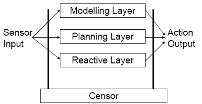
Reactive agents are built with a subsumption architecture, where organisation is by behavioural units (or layers), and decomposition is by activity, rather than decomposition by function. Each layer connects sensory input to effectors, and each layer is a reactive rule (originally implemented as an augmented finite state machine). Intelligent behaviour then emerges from the interation of many simple behaviours.
We can therefore say that the decision making of a reactive agent is realised through a set of task accomplishing behaviours. These behaviours are implemented as simple rules that map perceptual input directly to actions (state → action). As many rules can fire simultaneously, we need to consider a priority mechanism to choose between different actions.
We can formally specify a behaviour rule as a pair (c, a), where c ⊆ P is a condition and a is an action. A behaviour (c, a) will then fire when the environment is in state s ∈ S and c ⊆ See(s), that is, the agents' percepts in state s. We also let R be the set of an agents' behaviour rules, and we let '<' be a preference relation over R (a total ordering). We say that b1 < b2 is that b1 inhibits b2, i.e., that b1 will get priority over b2.
Reactive agents are therefore very efficient - there is a very small time lag between perception and action, simple and robust in noisy domains. We also say that they have cognitive adequacy. Humans have no full monolithic internal models, that is, no internal model of the entire visible scene, and they even have multiple internal representations that are not necessarily consistent. Additionally, humans have no monolithic control, and humans are not general purpose - they perform poorly in different contexts (especially abstract ones).
On the other hand, reactive agents require that the local environment has sufficient information for an agent to determine an acceptable action. They are hard to engineer, as there is no principled methodology for building reactive agents, and they are especially difficult to develop for complex environments.
We can therefore conclude that logic-based (symbolic) AI demonstrated sophisticated reasoning in simple domains, in the hope that these ideas can be generalised to the more complex domain, and nouvelle AI solved less sophisticated tasks in noisy complex domains, in the hope that this can be generalised to more sophisticated tasks. We should consider whether it is possible to get the best of both worlds.
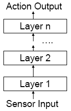
Layered Architectures
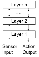
Layered architectures work by creating a subsystem (layer) for each type of behaviour (i.e., logic-based, reactive, etc) and these subsystems are arranged into a hierarchy of interacting layers. Horizontal layering is where each layer is directly connected to sensors and effectors, and vertical layering is where sensory input and output is dealt with by at most one layer each. Horizontal layering is shown below:
Vertical layering also comes in two varieties, one-pass control and two-pass control.
Multi-Agent Systems
Multi-agent systems come with the idea that "there is no single agent system". This is different to traditional distributed systems in that agents may be designed by different individuals with different goals, and agents must be able to dynamically and autonomously co-ordinate their activities and co-operate (or compete) with each other.
One methodology for multi-agent systems is co-operative distributed problem solving (CDPS). This is where a network of problem solvers work together to solve problems that are beyond their individual capabilities; no individual node has sufficient expertise, resources and information to solve the problem by themselves. CDPS works on the benevolence assumption that all agents share a common goal. Self-interested agents (agents designed by different individuals or organisations to represent their interests) can exist, however.
Multi-agent systems can be evaluated using two main criteria: coherence - that is, the solution quality and resource efficiency; and the co-ordination, the degree to which the agents can avoid interfering with each other, and having to explicitly synchronise and align their activities.
Issues in CDPS include dividing a problem into smaller tasks for distribution among agents, synthesising a problem solution from sub-problem results, optimising problem solving activities to achieve maximum coherence and avoiding unhelpful interactions and maximising the effectiveness of existing interactions.
Task and result sharing comes in three main phases: problem decomposition, where sub-problems (possibly in a hierarchy) are produced to an appropriate level of granuality; sub-problem solution, which includes the distribution of tasks to agents; and solution synthesis.
One way of accomplishing this is using a method known as contract net. This is a task sharing mechanism based on the idea of contracting in the business world. Currently, contract net is the most implemented and best studied framework for distributed problem solving.
Contract net starts by task announcement - an agent called a task manager advertises the existance of a task (either to a specific audience, or all), and agents listen to announcements, evaluate them and decide whether or not to submit a bid. A bid indicates the capabilities of the bidder with regard to the task. The announcer receives the bids and chooses the most appropriate agent (the contractor) to execute the task. Once a task is completed, a report is sent to the task manager.
The agents co-operatively exchange information as a solution is developed, and result sharing improves group performance in the following ways:
- confidence: independently derived solutions can be cross-checked
- completeness: agents share their local views to achieve a better global view
- precision
- timeliness: a quicker problem solution is achieved
A co-ordination mechanism is necessarily to manage inter-dependencies between the activities of agents. We can consider a hierarchy of co-ordination relationships:
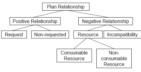
There are multiple types of positive, non-requested relationships:
- action equality relationship: two agents plan to perform an identical action, so only one needs to perform it
- consequence relationship: a side-effect of an agent's action achieves an explicit goal of another
- favour relationship: a side-effect of an agent's plan makes it easier for another agent to achieve his goals
Partial Global Planning
In partial global planning, the idea is that agents exchange information in order to reach common conclusions about the problem-solving process. It is partial as the system does not generate a plan for the entire problem, and is global as agents form non-local plans by exchanging local plans to achieve a non-local view of problem solving.
There are three stages in partial global planning. In the first, each agent decides what its own goals are and generates plans to achieve them. Agents then exchange information to determine where plans and goals interact. Agents then alter their own local plans in order to better co-ordinate their own activities.
A meta-level structure guides the co-operation process within the system. It dictates which agents an agent should exchange information with, and under what conditions information exchanges should take place.
A partial global plan contains: an objective which the multi-agent system is working towards; activity maps, which are a representation of what agents are actually doing, and what results will be generated by the activities; and a solution construction graph, which represents how agents ought to interact, what information ought to be exchanged, and when.
Finally we need to consider multi-agent planning. In a multi-agent system, we can either have centralised planning for distributed plans, distributed planning for centralised plans, or distributed planning for distributed plans. When planning is distributed, we need to consider plan merging.
Plan merging works by taking a set of plans generated by single agents, and from them generating a conflict-free multi-agent plan. This multi-agent plan is not necessarily optimal, however. We can use planning approaches discussed above, however we often also require a During List, which contains conditions that must hold whilst the action is being carried out.
Plan merging has three stages:
- interaction analysis, where interactions in between the agents' plans are discovered. This is based on the principles of: satisfiability, where two actions are said to be satisfiable if there is some sequence in which they may be executed without invalidating a pre-condition; commutativity, where two actions may be executed in parallel; and precedence, which is the sequence in which actions may be executed
- safety analysis, where it is determined which interactions are unsafe. Actions where there are no interaction, or where the actions commute, are removed from the plan, and the set of all harmful interactions is generated using search
- interaction resolution, which is the mutual exclusion of critical sections (i.e., unsafe plan interactions)