Machine Learning
A possible definition of machine leaning is the study of how to design computer programs whose performance at some task improves through experience.
Mitchell more precisely defines that a computer program is said to learn from experience E, with respect to some class of tasks T and performance measure P, if its performance at tasks in T as measured by P improves with experience E.
However, are we only interested in the performance of the learning program, or are we also interested in discovering human-comprehensible descriptions of patterns in data (knowledge discovery).
There are multiple motivations for studying machine learning: technological or engineering motivations (e.g., building computer systems that can improve their performance at tasks with experience), computer science motivations (e.g., to understand better properties of various algorithms for function approximation) and a cognitive science motivation (to understand better how humans learn by modelling the learning process).
Machine learning has historically been used for data mining (using historical data to improve decisions), developing software applications that can't be programmed by hand (particularly classification), or personalisation/adaptive programs (such as web advertising).
We must also consider that is to be learnt - typically it's a computational structure of some sort. Nilsson (1997) proposed that these could be functions, finite state machines, grammars or a problem solving system.
Input-Output Functions
Much machine learning is set in the context of learning input-output functions. This includes applications such as character and speech recognition, where a graphical representation of a character sequence or a waveform is taken and a character of word sequence is returned, face recognition, load forecasting for the National Grid, credit assessment or games.
We can consider learning a function as curve fitting - finding a function which closely approximates the data we have. If we are trying to learn a function f (or the target function) which takes a vector-valued input (typically an n-tuple) and f itself may be vector valued, yielding a k-tuple as output. Often f produces a single output value.
The job of the learner is to output a hypothesis h which is a guess or approximation of the target function f. We assume that h is drawn a priori from a class of function H. f is not always known, and is not necessarily in the class H.
The learner selects h based on a set of training examples. Each training example consists of an n-tuple x drawn from the set of input vectors over which f is defined.
If for each training example x the value of f (i.e., f x) is also supplied, then the learning setting is called a supervised learning setting (most of the methods covered here will be supervised). If the training examples do not have associated output values, then the learning setting is called unsupervised learning.
Unsupervised learning is just used to explore the data, and is useful for partitioning datasets. Supervised learning is more useful - you give it inputs and the expected ouputs to find the best f.
Input vectors go by a variety of names in the literature: input vector, pattern vector, feature vector, sample, example, instance, etc, and the components xi are variously called features, attributes, input variables or components. The values of components are generally of two major sorts: numeric (or ordinal - themselves in two divisions: real-valued and discrete-valued numbers) and nominal (or categorical, enumerated, or confusingly discrete).
If a learner produces a hypothesis h that outputs a real number, it is called a function estimator and its output is called an output value or estimate.
If a learner produces a hypothesis h that outputs a categorical value, it is called a classifier, or a recogniser categoriser, and its output is called a label, class, category or decision.
Outputs could also be vector-valued with the components being numeric and nominal (or both).
Training
When it comes to the training regimes, considerable variation is possible in how training examples are presented or used. In the batch method, all training examlpes are available and used all at once to compute h (in a variant of this, all training examples are used iteratively to refine a current hypothesis until some stopping condition). In the incremental method, one member of the training set is selected at a time and used to modify the current hypothesis. Members of training set can be selected at random, or cycled through iteratively. If training instances become available at a particular time and are used as soon as they become available, this is called an on-line method.
Training can be direct, where each training instance has an associated target value, or indirect where only sequences of training instances have an associated outcome (e.g., chess). It may not be possible to know if an individual move is correct, only whether a sequence of moves leads to win or loss. The learner must decide which moves in the sequence were good or bad (this is the credit assignment problem).
A final consideration is to know how well our learner is doing (i.e., how good the hypothesis it produces is). A standard approach is to test the hypothesis on a set of inputs and function values not used in training - this is called the test set. Common evaluation measures used are the mean-squared error and accuracy tests (e.g., the proportion of instances misclassified).
Concept Learning
Much learning is acquiring general concepts or categories from specific examples, which can more mathematically be viewed as a subset over a larger set (e.g., learning what a house is as a particular subset of human artifacts by specific examples in that subset) or as a boolean-valued function over a larger set (a function over human artifacts which is true for houses and false for other artifacts).
Mitchell defines concept learning as inferring a boolean-valued function from training examples of its inputs and output. Concept learning is also known as binary classification.
Specific examples are
in the lecture slides.
If we wanted to learn a target concept, then our input is a set of examples each describing the concept in the terms of a set of attributes and a positive or negative marker of whether that particular example is true for that concept. Using these examples, the task is to learn how to predict the positive or negative marker for a previously unseen set of attributes.
If we suppose that our hypotheses take the form of conjunctions on the instance attributes and suppose our constraints take one of three forms: ?, which means any value is acceptable, SpecifiedValue, which is a specific value of that attribute, or ∅ which means that no value is acceptable, then our hypotheses can be represented as vectors of such constrains.
This concept learning setting can be described as follows:
- Given X, a set of instances over which the concept is to be defined (each represented, e.g., as a vector of attribute values);
- a target function of concept to be learnt: (c : X → {0,1})
- and a set D of training examples, each of the form ⟨x, c(x), where x ∈ X and c(x) is the target concept value for x (note, instances in D where c(x) = 1 are called positive examples, and those for which c(x) = 0 are called negative examples).
- Find a hypothesis, or estimate, of c. (i.e., supposing H is the set of all hypothesis, find h ∈ H where h : X → {0,1} such that h(x) = c(x) ∀ x ∈ X).
Concept learning can this be viewed as a search over the space of hypotheses, as defined by the hypothesis representation.
We want to find h identical to c over all of X, but we only have the information about training examples D. Inductive learning algorithms can only guarantee that hypotheses fit training data, therefore we presume under the following assumption:
Any hypothesis found to approximate the target function well over a sufficiently large set of training examples will also approximate the target function well over other unobserved examples. (Mitchell definition of Inductive Learning Hypothesis).
General-to-Specific Hypotheses Ordering
Concept learning may be viewed as search over the space of hypotheses, as defined by the hypothesis representation, we can compute the number of distinct value combinations, and remember the combinations can include ? and ∅ to compute the number of syntactically distinct hypotheses.
However, since every hypotheses containing one or more ∅'s is equivalent (this classifies all instances as negative), we can reduce the number of syntactically distinct hypotheses to find the number of semantically distinct hypotheses.
We now have a problem of how to search this space to find the target concept.
One solution is to start with the most specific hypotheses (a vector of ∅) and, considering each training example in turn, generalise towards the most general hypothesis (a vector of ?), stopping at the first hypothesis that covers the training examples. This is called Find-S.
Intuitively we know that a hypothesis hi is more general than hj if every instance that hj classifies as positive, hi also classifies as positive, and hi classifies instances as positive that hj does not.
More formally, we say that instance x satisfies hypothesis h iff h(x) = 1. We define a partial ordering relation more-general-than-or-equa-to holding between two hypotheses hi and hj in terms of the sets of instances that satisfy them: hi is more-general-than-or-equal-to hj iff every instance that satisfies hj also satisfies hi.
Or, let hi and hj be boolean-valued functions defined over X. hi is more-general-than-or-equal-to hj (hi ≥g hj) iff (∀x ∈ X)[(hj(x) = 1) → (hi(x) = 1)].
≥g provides a strucutre over the hypothesis space H for any concept learning problem. Learning algorithms can take advantage of this.
Find-S
Find-S is used to find a maximally specific hypothesis, and the algorithm is defined as:
1. Initialise h to the most specific hypothesis in H
2. For each positive training instance x:
For each attribute constraint ai in h:
If the constraint ai in h is satisfied by x,
then do nothing
else replace ai in h by the next more general constraint satisfied by x
3. Output hypothesis h
Note that Find-S completely ignores negative training instances.
For hypothesis spaces described by conjunctions of attribute constraints, Find-S is guaranteed to output the most specific hypothesis in H consistent with the positive training examples. Find-S is also guaranteed to output a hypothesis consistent with the negative examples provided that the correct target concept is in H, and the training examples are correct.
However, Find-S has multiple problems. There may be multiple hypotheses consistent with the training data, but Find-S will only find one and give no indication of whether there may be others.
Find-S also always propose the maximally specific hypothesis, but why is this preferred to, for example, the maximally general? Find-S also has seriour problems when training examples are inconsistent - which frequently happens with noisy "real" data.
Version Spaces
One limitation of the Find-S algorithm is that it outputs just one hypothesis consistent with the training data, when there may be many. To overcome this, we can use version spaces and related algorithms to compute it.
A hypothesis h is consistent with a set of training examples D of a target concept c iff h(x) = c(x) for each training example ⟨x, c(x)⟩ in D:
Consistent(h, D) ≡ (∀⟨x, c(x)⟩ ∈ D)h(x) = c(x)
The version space, VSH,D, with respect to hypothesis space H and training examples D, is the subset of hypotheses from H consistent with all training examples in D.
VSH,D ≡ {h ∈ H | Consistent(h, D)}
It is important to note the difference between definitions of consistent and satisfies:
- an example x satisfies hypothesis h when h(x) = 1, regardless of whether x is a positive or negative example of a target concept;
- an example x is consistent with an hypothesis h iff h(x) = c(x).
List-Then-Eliminate
One way to represent the version space is by listing all of its members, which leads to the list-then-eliminate concept learning algorithm:
1. VersionSpace ← a list containing every hypothesis in H
2. For each training example ⟨x, c(x)⟩ remove from VersionSpace any hypothesis h for which h(x) ≠ c(x)
3. Output the list of hypotheses in VersionSpace
List-then-eliminate works in principle, so long as the version space is finite, however, since it requires an exhaustive enumeration of all hypotheses, in practice it is not feasible. From this, we can consider a more compact way to represent version spaces.
Candidate-Elimination
The candidate-elimination algorithm is similar to the list-then-eliminate algorithm, but uses a more compact representation of version space - representing it by its most general and most specific members. Other intermediate members in a general-to-specific ordering can be generated as needed.
The general boundary, G, of the version space VSH,D is the set of its maximally general members. The specific boundary, S, of version space VSH,D is the set of its maximally specific members.
Mitchell p.32 has a proof
The version space representation theorem states that every member of the version space lies between these boundaries: VSH,D = {h ∈ H | (∃s ∈ S)(∃g ∈ G)(g ≥g h ≥g s)}
Intuitively, the candidate-elimination algorithm proceeds by initialising G and S to the maximally general and maximally specific hypotheses in H, and then considering each training example in turn: use positive examples to drive the maximally specific boundary up, and use negative examples to drive the maximally general boundary down.
More formally we can specify this as:
G ← maximally general hypotheses in H
S ← maximally specific hypotheses in H
For each training example d:
if d is a positive example:
Remove from G any hypotheses inconsistent with d
For each hypotheses s in S that is not consistent with d:
Remove s from S
Add to S all minimal generalisations h of s such that h is consistent with d and some member of G is more general than h
Remove from S any hypothesis that is more general than another hypothesis in S
if d is a negative example:
Remove from S any hypotheses inconsistent with d
For each hypotheses g in G that is not consistent with d:
Remove g from G
Add to G all minimal generalisations h of g such that h is consistent with d and some member of S is more specific than h
Remove from G any hypothesis that is less general than another hypothesis in S
The version space learned by the candidate-elimination algorithm will converge towards a central hypothesis provided there are no errors in the training examples, and there is a hypothesis in H that describes the target concept. In such cases, the algorithm will converge to an empty space.
If the algorithm can request the next training example (e.g., from a teacher), the speed of convergence can be increased by requesting examples that split the version space. an optimal query strategy is to request examples that exactly split the version space - this would converge in ⌈log2 |VS|⌉ steps, however this is not always possible.
When using a classifier that has not completely converged, new examples may be classed as positive by all h ∈ VS, classes as negative by all h ∈ VS, or classed as positive by some, and negative by others.
The first two cases here are unproblematic, but in case 3, we may want to consider the proportion of positive vs. negative classifications (but then a priori probabilities of hypotheses are relevant).
Inductive Bias
As noted, the version space learned by the candidate-elimination algorithm will converge towards the correct hypothesis provided that there are no errors in the training examples, and there is a hypothesis in H that describes the target concept - however, what if no concept in H describes the target concept?
A more expressive hypothesis representation language is needed, specifically to allow disjunctive or negative attribute values.
An unbiased learned would ensure that every concept can be represented in H. Since concepts are subsets of an instance space X, we want H to be able to represent any set in the power set of X.
We can do this by allowing hypotheses that are arbitrary conjunctions, disjunctions and negations of our earlier hypotheses, but we have a new problem: the concept learning algorithm can not generalise beyond the observed examples - the S boundary is a disjunction of positive examples (covering exactly the observed positive examples) and the G boundary is a negative of a disjunction of negative examples (exactly ruling out the observed negative examples).
The capacity of candidate-elimination to generalise lies in its implicit assumption of bias - that the target concept can be represented as a conjunction of attribute values.
This forms a fundamental property of inductive inference: A learner that makes no a priori assumptions regarding the identity of the target concept has no rational basis for classifying any unseen instances (i.e., bias-free learning is futile).
More formally, since all inductive learning involves bias, it is useful to characterise learning approaches by the type of bias they employ.
If we consider a concept learning algorithm L, some instances X and a target concept c and the training examples Dc = {⟨x, c(x)⟩}, then let L(xi, Dc) denote the classification, positive or negative, assigned to the instance xi by L after training data on Dc. The inductive bias of L is any minimal set of assertions B such that for any target concept c and corresponding training examples Dc:
(∀xi ∈ X)[(B ∧ Dc ∧ xi) |- L(xi, Dc)].
Decision Tree Learning
Decision trees are trees which classify instances by testing at each node some attribute of the instance. Testing starts at the root node and proceeds downwards to a leaf node, which indicates classification of the instance. Each brand leading out of a node corresponds to a value of the attribute being tested at that node.
Each path through a decision tree forms a conjunction of attribute tests, and the tree as a whole forms a disjunction of such paths (i.e., a disjunction of conjunctions of attribute tests).
For complex rules, some decision trees could be coded by hand, but the challenge for machine learning is to propose algorithms for learning decision trees from examples.
There are several varieties of decision tree learning, but in general decision tree learning is best for problems where:
- instances are describable by attribute-value pairs, usually nominal (categorical/enumerated/discrete) attributes with a small number of discrete values, but it can be numeric (ordinal/continuous);
- the target function is discrete valued (e.g., boolean, but easy to extend to target functions with >2 output values). It is possible, but harder, to extend to numeric target functions;
- a disjunctive hypothesis may be required - it is easy for decision trees to learn disjunctive concepts (which were outside the hypothesis space of the candidate-elimination algorithm we've covered before);
- the training data is possibly noisy or incomplete. Decision trees are robust to errors in classification of training examples and errors in attribute values describing these examples, and can also be trained on examples where some instances of the attribute values are unknown.
ID3
The ID3 algorithm (originally called binary classification) is the basic decision tree learning algorithm:
ID3(Examples, Target_Attribute, Attributes):
Create a root node for the tree
If all examples positive, return 1-node tree Root with label +
Else if all examples negative, return 1-node tree Root with label -
Else if Attributes = [] return 1-node tree Root with the label of the most common value of Target_Attribute in Examples
Else
A ← the attribute in Attribues that best classifies Examples
The decision attribute for Root ← A
Let Examplesvi = subset of Examples with value vi for A
If Examplesvi = []
Then below this new branch add leaf node with label = the most common value of Target_Attribute in Examples
Else below this new branch add the subtree ID3(Examplesvi, Target_Attribute, Attributes - {A})
Return Root
Information Gain
Choosing which attribute to test at the next node is a crucial step in ID3. We would like the choose the attribute which does best at separating training examples according to their target classification. An attribute which separates training examples into two sets, each of which contains positive and negative examples of the target attribute in the same ratio as the initial set of examples has not helped us progress towards a classification.
A useful measure for picking the best classifier attribute is information gain. Information gain measures how well a given attribute separates training examples with respect to their target classification.
Entropy
Information gain is defined in terms of entropy as used in information theory. If S is a sample of training examples, p+ is the proportion of positive examples in S and p- is the proportion of negative examples in S, then entropy measures the impurity of S: entropy(S) ≡ -p+log2 p+ - p-log2p-.
We can think of Entropy as the expected number of bits needed to encode a class (+ or -) or randomly drawn members of S (under the optimal, shortest-length code).
- If p+ = 1 (i.e., all instances are positive), then no message need be sent (the receiver knows the example will be positive) and Entropy = 0, a pure sample;
- If p+ = 0.5, then 1 bit need be sent to indicate whether instance is negative or positive and Entropy = 1;
- If p+ = 0.8, then less than 1 bit needs to be sent on average - shorter codes are assigned to collections of positive examples, and longer ones to negative ones.
Entropy gives a measure of purity/impurity of a set of examples. Information gain is defined as the expected reduction in entropy resulting from partitioning a set of examples on the basis of an attribute.
Formally, given a set of examples S and an attribute A: Gain(S, A) ≡ Entropy(S) - Σv ∈ Values(A) ((|Sv| / |S|) Entropy(Sv), where Values(A) is the set of values attribute A can take on, and Sv is the subset of S for which A has value v.
The first term in Gain(S,A) is the entropy of the original set, and the second term is the expected entropy after partitioning on A (the sum of entropies of each subset Sv weighted by the ratio of Sv in S).
ID3 searches a space of hypotheses (a set of possible decision trees) for one fitting the training data. The search is a simple-to-complex hill-climbing search guided by the information gain evaluation function.
The hypothesis space of ID3 is a complete space of finite, discrete-valued functions with regard to available attributes (as opposed to an incomplete hypothesis space, such as the conjunctive hypothesis space).
ID3 maintains only one hypothesis at any time, instead of (e.g.) all hypotheses consistent with the training examples seen so far. This means it can't ask questions to resolve competing alternatives, or determine how many alternative decision trees are consistent with the data.
ID3 performs no backtracking - once an attribute is selected for testing at a given node, this choice is never reconsidered, so it is susceptible to converging to local optima, rather than globally optimum solutions. It also uses all training examples at each step to make statistically-based decisions about how to refine the current hypothesis (as opposed to Candidate-elimination or Find-S, which makes decisions incrementally based on single training examples). Using statisically based properties of all the examples means this technique is robust in the face of errors in individual examples.
Inductive Bias
Recall that inductive bias is the set of assumptions needed in addition to training data to justify the learners classifications.
Given a set of training examples, there may be many decision trees consistive with them, so the inductive bias of ID3 is shown by which of these trees is chooses.
ID3's search strategy (simple-to-complex hill-climbing) selects shorter trees over longer ones, and selects trees that place attributes with the highest information gain closest to the root.
ID3's inductive bias is therefore: shorter trees are preferred over longer trees, and trees that place high information gain attributes close to the root are preferred to those that do not.
A decision tree learning algorithm could be produced with the simpler bias of always preferring a shorter tree, e.g., an algorithm that started with the empty tree and did a breadth-first search through the space of all decision trees, but this suffers from an issue of no bias, and also an increase in time and space complexity.
Compared to candidate-elimination, we can say that ID3 incompletely searches a complete hypothesis space, and candidate-elimination completely searches an incomplete hypothesis space.
The inductive bias of ID3 comes from its search strategy (called preference or search bias), whereas the inductive bias of candidate-elimination follows from its definition of its search space (restriction or language bias).
Preference bias affects the order in which hypotheses are investigated; restriction bias affects which hypotheses are investigated. It is generally better to choose an algorithm with a preference bias than a restriction bias - with a restriction bias, the target function may not be in the hypothesis space. Some algorithms combine preference and restriction biases.
We should also ask ourselves if ID3's inductive bias is sound - why should we prefer shorter hypotheses/trees? One argument favoured by natural scientists is the principle of Occam's Razor. In favour of this principle one can argue that there are fewer short hypotheses than long hypotheses, and a short hypothesis that fits the data is less likely to be a coincidence than a long hypothesis which does the same. However, there are many ways to define small sets of hypotheses, and we should consider what's so special about small sets based on the size of the hypothesis?.
Overfitting
If we got a new example whose target classification is wrong, then the result will be a tree that performs well on errorful training examples, but less well on new unseen instances. Adapting to this noisy training data is one type of overfitting.
Overfitting can also occur when the number of training examples is too small to be representative of the true target function, and coincidental regularities can be picked up during training.
More precisely, we say that given a hypothesis space H, a hypothesis h ∈ H overfits the training data if there is another hypothesis h′ ∈ H such that h has a smaller error than h′ over the training data, but h′ has a smaller error over the entire distribution of instances.
Overfitting is a real problem for decision tree learning, with one empirical study showing a 10-25% decrease in accuracy over a range of tasks. Other machine learning tasks also suffer from the problem of overfitting.
There are two approaches to avoiding overfitting: stopping growing trees before it perfectly fits the training data (e.g., when the data split is not statistically significant), or to grow the full tree and then prune it afterwards. In practice, the second approach is more successful.
For either approach, we have to find the optimal final tree size. Ways to do this include using a set of examples distinct from the training examples to evaluate the quality of the tree, using all the data for training but then applying a statistical test to decide whether expanding or pruning a given node is likely to improve performance over the whole instance distribution, or measuring the complexity of encoding the exceptional training examples and the decision tree, and to stop growing the tree when this size is minimised (the minimum description length principle).
The first approach is the most common and is called the training and validation set approach. Available instances are divided into a training set (approximately 2/3rds of the data) and a validation set (commonly around 1/3rd of the data) with the hope that random errors and coincidental regularities learned from the training set will not be present in the validation set.
With this approach, assuming the data is split into the training and validation sets, we train the decision tree on the training set, and then until further pruning is harmful, for each decision node we evaluate the impact on the validation set of removing that node and those below it, and then remove the node that most improves the accuracy on the validation set.
The impact of removing a node is evaluated by removing a decision node, and the subtree rooted at it is replaced with a leaf node whose classification is the most common classification of the examples beneath the decision node, and this new tree can be evaluated.
To assess the value of reduced error pruning, we can split the data into 3 distinct sets: the training examples for the original tree, the validation examples for guiding the tree pruning, and further test examples to provide an estimate over future unseen examples. However, holding data back for a validation set reduces the data available for training.
Rule post-pruning is perhaps the most frequently used method (e.g., in C4.5).
This proceeds by converting the tree to an equivalent set of rules (by making the conjunction of decision nodes along each branch the antecedent of a rule, and each leaf the consequent), pruning each rule independently of the others, and then sorting the final rules into a desired sequence for use.
To prune rules, any precondition (the conjunct in an antecedent) of a rule is removed, if it does not worsen rule accuracy. This can be estimated by using a separate validation set, or by using the training data but assuming a statistically-based pessimistic estimate of rule accuracy (C4.5 does the latter).
By converting trees to rules before pruning, this allows us to distinguish different contexts in which rules are used, and to therefore treat each path through the tree differently (in contract to removing a decision node, which removes all the paths below it). Also, this removes the distinction between testing nodes near the root, and those near the leaves, avoiding the need to rearrange the tree should higher nodes be removed. Rules are often easier for people to understand too.
Continuous-valued attributes
The initial definition of ID3 was restricted to discrete-valued target attributes and decision node attributes.
We can overcome this second limitation by dynamically defining new discrete-valued attributes that partition a continuous attribute value into a set of discrete intervals, i.e., for a continuous value A, we dynamically create a new boolean attribute Ac that is true if A > c and false otherwise. c is chosen such that it maximises information gain. This can be extended to split continuous attributes into more than 2 intervals.
The information gain measure favours attributes with many values other those with few values - e.g., a date attribute would result in a tree of depth 1 that perfectly classifies the training examples but fails on all other data, because date perfectly predicts the target attribute for all training examples.
Other attribute selection measures can be used to avoid this.
One such measure is gain ratio: GainRatio(S,A) ≡ Gain(S,A) / SplitInformation(S,A), such that SplitInformation(S,A) ≡ -Σci = 1 ( (|Si| / |S|) log2 (Si / |S|) ), where Si is a subset of S for which the c-valued attribute A has the value vi. SplitInformation is the entropy of S with regard to the values of A. This has the effect of penalising attributes with many uniformly distributed values.
Experiments with variants of this and other attribute selection techniques have been carried out and are reported in maching learning literature.
Another refinement to consider is in the case of missing values for some attribute in a training example. Several ways of handling this has been explored: At the decision node n where Gain(S,A) is computed, then either:
- assign the most common value of A among the other examples sorted to node n, or;
- assign the most common values of A among other examples at n with the same target attribute value as x, or;
- assign the probability pi to each possible value vi of A estimated from the observed frequencies of values of A for the examples sorted to A, or;
- assign the fraction pi of x distributed down each branch in the tree below n (this is technique used in C4.5).
The last technique can be used to classify new examples with missing attributes (i.e., after learning) in the same fashion.
Sometimes, different attributes can have different costs associated with acquiring their values (e.g., in medical diagnosis where different attributes have different costs), so it is beneficial to learn a consistent tree with a low expected cost.
Various approaches have been explored in which the attribute selection method is modified to include a cost term: e.g., Tan and Schlimmer's Gain2(S,A) / Cost(A) or Nunez's (2Gain(S,A) - 1) / (Cost(A) + 1)w, where w ∈ [0,1] which determines the importance of the cost.
Hypothesis Evaluation
Given a machine learning algorithm and a hypothesis h which it has learned from a set of examples, evaluating h allows us to evaluate how reliable h is in cases such as medical diagnosis, or for refinement of h (e.g., for post-pruning decision trees to avoid overfitting).
There are two potential problems in estimating the accuracy of an hypothesis h, specifically if the training or test data is limited:
- Bias in estimate - the observed accuracy of h on training data is not a good guide to future accuracy, as such an estimate is biased in favour of h. To get a good estimate of accuracy of h, we must test h on a sample chosen independency of the training set;
- Variance in estimate - even assuming an unbiased test sample, the resulting accuracy may still vary from the true accuracy depending on the makeup of the test set.
When evaluating an hypothesis, we want to know how accurately is will classify future instances, and how accurate our estimate of this accuracy is (i.e., what's the margin of error associated with our estimate).
The true error of a hypothesis h, with respect to a target function f and distribution D, is the probability that h will misclassify an instance drawn at random according to D: errorD(h) ≡ Prx ∈ D [f(x) ≠ h(x)].
The sample error of h with respect to target function f and data sample S is the proportion of examples h misclassifies: errorS(h) ≡ 1/n Σx ∈ S δ(f(x), h(x)), where n is the number of samples and δ(f(x), h(x)) is 1 if f(x) ≠ h(x) and 0 otherwise.
We want to know the true error, but we can only mesasure the sample error with respect to some sample S, so we need to know how well errorS(h) estimates errorD(h).
Lecture 6 contains
the justification for this.
Statistical theory tells us so long as the n instances in S are drawn independently of one another, independently of h, according to a probability distribution D and n >e; 30, then the most probable value of errorD(h) is errorS(h). With approximately N% probability, errorD(h) lies in the interval errorS(h) ± zN √, where zN = 0.67 for N = 50%, 1.00 for N = 68%, 1.28 for N = 80%, 1.64 for N = 90%, 1.96 for N = 95%, 2.33 for N = 98% and 2.58 for N = 99%.
Two and One-sided Bounds
The confidence intervals discussed so far only offer two-sided bounds - above and below, but we may only be interested in a one-sided bound (e.g., the upper bound on an error), and not mind if the error is lower than our estimate.
Since the normal distribution is symmetrical, we can convert any two-sided confidence interval into a one-sided interval with twice the confidence, e.g., we turn an 80% confidence interval into a 90% one-sided confidence interval by simply removing the lower bound (where an additional 10% lay).
Central limit theorem can be
user as a general approach to
deriving confidence intervals.
To derive a confidence interval for many estimation problems, we pick a paramater p to estimate (e.g., the errorD(h) - error of the hypothesis over the whole dataset), an estimator (errorS(h) - the error of the hypothesis over our sample), and then determine the probability distribution that governs the estimator (e.g., errorS(h) is governed by the Binomial distribution, so is normal when n >e; 30), and then find the interval (Lower, Upper) such that N% of the probability mass falls in the interval (e.g., using the zN values).
Things are made easier if we pick an estimator that is the mean of some sample, then (by Central Limit Theorem) we can ignore the probability distribution underlying the sample and approximate the distribution governing the estimator by the normal distribution.
We can also compare two learning algorithms rather than two specific hypotheses. There isn't complete agreement in the machine learning community about the best way to do this, but one way is to determine whether a learning algorithm LA is better on average (the relative performance of all training sets of size n drawn from the instance distribution D) for learning a target function f than a learning algorithm LB.
However, we have the issue of finding a good estimator given limited data. One way is to partition this into a training set and a test set, and measure the error of each algorithm trained on the same training set and tested with the same test set, or even better, repeating this many times and averaging the results.
Rather than dividing the limited training/testing data just once, we can do so multiple times and average the results. This is called k-fold cross-validation:
Partition data D0 into k disjoint test sets T1, ..., Tk of equal size, where this size is at least 30
For i from 1 to k:
Si ← {D0 - Ti}
δi ← errorTi(hA) - errorTi(hB)
Return , where = 1/k Σki = 1 δi
This isn't an estimate of error over the entire dataset, just a sample of it drawn uniformly from D0, but this approximation is better than nothing.
We can determine approximate N% confidence intervals for an estimator using a statistical test called a paired t test. A paired test is one where hypotheses are compared over identical samples, and uses the t-distribution rather than the normal distribution.
Another paired test in use is called the Wilcoxon signed rank test, which is non-parametric (does not assume any particular underlying distribution).
Additionally, rather than partitioning the available data into k disjoint equal sized partitions, we can repeatedly random select a test set of n >e; 30 examples from D0 and use the rest for training, doing this indefinitely many times to shrink the confidence intervals to an aribitrary width - however, test sets are no longer independently drawn from the underlying instance distibution, since instances will recur in separate test sets. In k-fold cross validation, each instance is only included in one test set.
So far we've assumed that the best measure of a learning algorithm is its error rate - but this is not always true. A classifier that always predicts positive on a set with sparse negative instances (e.g., 995 positive to 5 negative in a dataset of 1000) will have accuracy of 99.5%, but never correctly predict positive examples.
Confusion matrices allows deeper insight into classifier behaviour - it shows false negatives, false positives, true positives and true negatives.
| Predicted | |||
| Negative | Positive | ||
| Actual | Negative | a | b |
| Positive | c | d | |
From a confusion matrix, we can define the accuracy measure as defined earlier as (a + d)/(a + b + c + d), and other measures can also be defined.
Recall, or true positive rate, or sensitivity, is the proportion of positive cases that were correctly identified: d/(c + d), and the false positive rate as the proportion of negative cases incorrectly classified as positive: b/(a + b).
The true negative rate (or specifity) is defined as the proportion of negative cases that were classified correctly: a/(a + b), and conversely the false negative rate is the proportion of positive cases that were incorrectly classified as negative: c/(c + d).
Precision is the proportion of the predicted positive cases that were correct: d/(c + d).
To overcome the problems associated with accuracy as a sole measure, we always compare with the base, or baseline accuracy - the result of always predicting the majority class: max(a + b, c + d)/(a + b + c + d).
Other measures can also be used which take true positives into account, e.g., the geometric mean (√ or √), or the harmonic mean/f-measure.
Accuracy ignores the possibility of different misclassification costs (incorrectly positive costs may be more or less important than incorrectly predicting negative costs, e.g., in treatment of patients). To address this, many classifiers have parameters that can be adjusted to allow an increased TPR at the cost of an increased FPR, or vice versa.
For each such paramater setting of a (TPR, FPR) paid, the results may be plotted on an ROC (receiver operating characteristic) graph, which provides a graphical summary of trade-offs between sensitivity and specificity, arising from signal detection theory.
Bayesian Methods
Bayesian methods have two distinct important roles in machine learning: they provide practical learning algorithms which explicitly manipulate probabilities (naive Bayes learning and Bayesian belief network learning), and they provide a useful conceptual framework.
A significant feature of Bayesian learning algorithms is that they allow us to combine prior knowledge with observed data. Bayesian methods also provide a gold standard for evaluating other learning algorithms, and allow for additional insight into Occam's razor, and the inductive bias of decision tree learning in favour of short hypotheses.
COM6150 covers maximum a
posteriori and naive Bayes.
Bayes Theorem and Concept Learning
In some cases, it may be useful to assume that every hypothesis is equally probably a priori, i.e., P(hi) = P(hj) for all hi, hj ∈ H.
In such cases, we need only consider P(D|h), the likelihood of data D given h, to find the most probably hypothesis. Any hypothesis that maximises P(D|h) is called a maximum likelihood (ML) hypothesis: hML = argmaxh ∈ HP(D|h).
A brute force MAP hypothesis learner could be implemented like so: for each hypothesis h in H, calculate the posterior probability P(h|D) = P(D|h)P(h)/P(D), and then output the hypothesis hMAP with the highest posterior probability.
However, this brute-force MAP learning algorithm may be computationally infeasible, as it requires applying the Bayes theorem to all h ∈ H. However, this is still useful as a standard against which other concept learning approaches may be judged.
Therefore, to apply the brute-force MAP to concept learning, we assume that the training data is noise free, and that the target concept c is in hypothesis space H, and there is no a priori reason to believe any one hypothesis is more probable than any other. Therefore, we should choose P(h) = 1/|H| for all h ∈ H, therefore P(D|h), the probability of observing the target values D = ⟨d1, ..., dm⟩ for fixed instances ⟨x1, ..., xm⟩ if h is true is 1 if di = h(xi) for all di ∈ D, and 0 otherwise.
Therefore, the brute force algorithm can now proceed in two ways. If h is inconsistent with D, then P(D|h) = 0, therefore P(h|D) = 0, or h is consistent with the training data D and P(D|h) = 1, and P(h|D) = 1/|VSH,D|.
Therefore, if we assume a uniform prior probability distribution over H (i.e., P(hi) = P(hj, 1 ≤ i, j ≤ |H|) and deterministic, noise-free data (i.e., P(D|h) = 1 if D and h are consistent; 0 otherwise), then Bayes theorem tells us P(h|D) = 1/|VSH,D| if h is consistent with D, and 0 otherwise.
Thus, every consistent hypothesis has posterior probability 1/|VSH,D| and is a MAP hypothesis. One way of thinking of this is the posterior probability evolving as the training examples are presented from an initial even distribution over all the hypotheses to a concentrated distribution over those hypotheses consistent with the examples.
Consistent Learners
A consistent learner is any learner that outputs a hypothesis that commits 0 errors over the training examples. Each such learner, under the two assumptions of a uniform prior probability distribution over H and deterministic noise-free data, outputs a MAP hypothesis.
If we consider Find-S, as it outputs a consistent hypothesis (i.e., is a consistent learner), then under the assumptions about P(h) and P(D|h), Find-S outputs a MAP hypothesis. Find-S itself does not explicitly manipulate probabilities, but using a Bayesian framework, we can analyse it to show that its outputs are MAP hypotheses by identifying the underlying probability distributions P(h) and P(D|h) (analogous to characterising ML algorithms by their inductive bias).
Real Valued Functions
We can use Bayesian analysis to show, under certain assumptions, that any learning algorithm that minimises the squared error between hypothesis and training data in learning a real-valued function will output a maximum likelihood hypothesis.
If we consider any real-valued target function f and training examples ⟩xi, di⟨, where di is a noisy training value di = f(xi) + ei, where ei is a random variable (noise) drawn independently for each ei according to some normal distribution with mean = 0.
This is justified on slide 16.
The maximum likelihoold hypothesis is therefore the one that minimises the sum of the squared errors: hML = argminh∈HΣmi=1(di - h(xi))2.
Minimum Description Length
The Minimum Description Length (MDL) principle is the principle that shorter encodings (e.g., of hypotheses) are to be preferred. It too can be given an interpretation in the Bayesian framework.
MDL says (in a machine learning setting) hMDL = argminh∈HLC1(h) + LC2(D|h), where LC(x) is the description length of x under encoding C (i.e., prefer the hypothesis that minimises the length of encoding the hypothesis, plus the data encoded using the hypothesis).
LC1(h) is the number of bits to describe a tree h, and LC2(D|h) is the number of bits to describe D given h (and is equal to 0 is the examples are perfectly classified by h, so is only used to describe the exceptions), hence hMDL trades off tree size for training errors.
Bayes Optimal Classifier
So far we have sought the most probable hypothesis given the data D (i.e., hMAP), but given a new instance x, hMAP(x) is not the most probable classification.
In general, the most probable classification of a new instance is obtained by combining the predictions of all hypotheses, weighted by their posterior probability.
If we suppose that classifications can be any value vj from a set of values V, then the probability that P(vj|D) is the correct classification is Σhi∈HP(vj|hi)P(hi|D).
So, the optimal classification for a new instance is the value vj which maximises P(vj|D). This is the Bayes optimal classification: argmaxvj∈VΣhi∈HP(vj|hi)P(hi|D).
A surprising consequence of this is that Bayesian optimal classifiers may make predictions corresponding to hypotheses not in H (i.e., the classifications over all x in X produced by a Bayesian classifier may not be those which any single hypothesis in H would produce). Hence, we can think of the Bayesian optimal classifier operating over a hypothesis space H′, which includes the hypotheses that perform linear combinations of multiple hypotheses in H, and is different to the H over which Bayes theorem is applied.
Gibbs Algorithm
The Bayes optimal classifier provides the best classification result achievable, however it can be computationally intensive, as it computes the posterior probability for every hypothesis h ∈ H, the prediction of each hypothesis for each new instance, and the combination of these 2 to classify each new instance.
Gibbs chooses one hypothesis at random according to P(h|D), and uses this to classify a new instance.
If we assume the target concepts are drawn at random from H according the the priors on H, then the error of Gibbs is less than twice the error of optimal Bayes.
Gibbs is seldom used, however.
Bayesian Belief Networks
The assumption which underlies the naive Bayes classifier, that attribute values are conditionally independent given some target value, this works fine in some settings, but in others it is too restrictive.
However, Bayesian classification is intractable without some assumption. Bayesian belief networks are some sort of intermediate approach. Rather than obliging us to determine dependencies between all the combinations of attributes/attribute values they describe the conditional independence among subsets of attributes.
More precisely, if we think of the attributes as discrete-valued random variables Y1, ..., Yn, each of which takes on a value from a set of values Vi, then the joint space of the variables is V1 × ... × Vn and the joint probability distribution is the probability distribution over this space.
Bayesian belief networks describe a joint probability distribution for a set of variables, typically a subset of available instance attributes, and allow us to combine prior knowledge about dependencies and independencies among attributes with the observed training data.
Bayesian belief networks are represented as a directed acyclic graph, where each node represents a variable, and the directed arcs represent the assertion that the variable is conditionally independent of its non-descendants, given its immediate predecessors. Associated with each variable is a conditional probability table describing the probability distribution for that variable, given the values of its immediate predecessors.
The network completely describes the joint probability distribution of the variables represented by its nodes, according to the formula P(y1, ..., yn) = &product;ni=1 P(yi | Parents(Yi)), where Parents(Yi) denotes the immediate predecessors of Yi in the graph.
CPTs work well for networks where all of the variables are discrete, but if the network contains continuous variables, it is impossible to specify conditional probabilities explicitly for each value - there are infinitely many values. One approach to avoid continuous variables is using discretisation - dividing up the data into a fixed set of intervals. This sometimes works, but can result in a loss of accuracy and very large CPTs.
Another approach is to use standard families of probability density functions that are specified by a finite number of parameters (e.g., normal or gaussian).
Bayesian networks where conditional distribution for a continuous variable given a discrete or continuous parents, and conditional distribution for a discrete variable given continuous parents need to be addressed.
To infer the probabilities of the values of one or more network variables given the observed values of the others can be done using Bayesian networks.
If only one variable (the query variable) is unknown, and all other variables have observed values, then it is easy to infer, but in the general case, there may be unobserved, or hidden, variables in addition to the observed or evidence variables. What is then sought, for each query variable X and observed event e (where e instantiates a set of evidence variables), is the posterior probability distribution P(X|e). This problem is NP-hard.
This can succeed in many cases, however. Exact inference methods work well for some network structures, and for large, multiply connected networks, approximate inference can be carried out using randomised sampling, or Monte Carlo, algorithms, which provide approximate answers whose accuracy depends on the number of samples generated.
Learning Bayesian Networks
Learning Bayesian networks have a number of aspects: e.g., whether the structure is known or unknown, and whether the training examples provide values of all network variables, or just some (i.e., the variables may be observable or hidden).
Russel and Norvig p.719-720
for info on continuous network variables.
If the network structure is known, and we can observe all variables, then the probabilities for the CPTs can be estimated directly from the training data. This is straightforward is all network variables are discrete, but more complex is any network variables are continuous (we would need to estimate the parameters, e.g., using a linear Gaussian model).
Including hidden variables in the model allows us to greatly reduce the complexity of the Bayesian networks, so it is generally useful to include them using the minimum description length principle, and also reducing the number of parameters in the conditional distribution, in turn reducing the amount of data required to learn the parameters.
Various methods have been explored for learning parameters of hidden variables in Bayesian nets - one of the most popular methods is to use the expectation-maximisation (EM) algorithm.
The general EM framework is that, given data with missing values, the space of possible models and an initial model, then until there is no change greater than the threshold, repeat the expectation step (compute the expectation over the missing values, given the model) and the maximisation step (replace the current model with a model that maximises the probability of data).
EM is not just used for parameter estimation for hidden variables in Bayesian nets, for in many other applications, including unsupervised data clustering and hidden Markov models.
So far, we have assumed the structure of the network is known, which frequency reflects the basic causal knowledge about the domain, but in some cases, the causal model is not available or is in dispute. When the Bayesian network structure is unknown, we can search for a good model.
Starting with a model with no links, we add the parents for each node, fit some parameters and the measure the accuracy of the resulting model, or, we can guess the initial structure and use some algorithm (e.g., a hill-climbing one) to add/subtract/reverse edges and nodes.
Additionally, a method is needed for deciding when a good structure has been found. We can test whether the conditional independence assertions implicit in the structure are satisfied in the data, and we can measure the extent to which the proposed model explains the data - however we must be careful to penalise complexity, since trying to find the maximum-likelihood hypothesis will lead to a fully connected network, as adding more parents can not decrease likelihood. This is an active research topic.
Instance-based Learning
Instance-based methods simply store the training examples, and when a new instance is to be classified, it is compared to the stored examples, and depending on its relationship to them, assigned a target classification.
Instance-based methods are called lazy methods, as they defer processing until a new instance is classified. Methods which build representations of the target function as training examples are presented are called eager methods.
Lazy methods trade-off training time computation with classification time computation, and can form local rather than global approximations to the target function, where the approximation could be separate for each new query instance.
Lazy methods may consider the query instance in deciding how to generalise beyond the training data - eager methods can not.
k-nearest neighbour learning
k-nearest neighbour, or k-NN is the grandad of instance-based methods. It generally assumed that instances are represented as n-tuples of real values, i.e., as points in n-dimensional space Rn.
The distance between any two instances is defined in terms of Euclidean distance, so given an instance x described by ⟨a1(x), ... an(x)⟩, where ar(x) is the value of the rth attribute of x, then the distance between the two instances xi and xj is defined as d(xi, xj) = √.
Given a new instance xq to classify, k-NN finds the nearest k instances closest to xq according to the distance measure d and picks their most common value for discrete-valued target functions, and picks their mean value for real-valued target functions. It can be thought of as nearest neighbours voting for the classification of the query instance.
Some variants interpret k as the k nearest distances instead of the k nearest instances to account for multiple equidistant neighbours.
For discrete-valued target functions f : X → V, the algorithm is:
If training, for each training example ⟨x, f(x)⟩, add the example to the list training_examples
If classifying, given a query instance xq to be classified:
Let x1,x2, ..., xk denote the k nearest instances in training_examples to xq
return f^(xq) ← argmaxv ∈ V∑ki=1 δ(v, f(xi)), where δ(a, b) = 1, if a = b and δ(a, b) = 0 otherwise.
For continous-valued target functions f : X → R:
If training, for each training example ⟨x, f(x)⟩, add the example to the list training_examples
If classifying, given a query instance xq to be classified:
Let x1,x2, ..., xk denote the k nearest instances in training_examples to xq
Return f^(xq) ← (∑ki=1f(xi))/k
Distance weighted k-nearest neighbour
k-NN can be refined by weighting the contribution of k neighbours according to their distance from the query instance xq, i.e., closer neighbours count more, further neighbours count less.
This can be achieved by changing the calculation in the classification step of the basic k-NN algorithm for discrete-valued target functions, e.g., weighting the vote of each of the k-NN according to the inverse square of its distance from xq:
f^(xq) ← argmaxv ∈ V∑ki=1 δ(v, f(xi)), where wi = 1/(d(xq, xi)2).
For continuous-valued target functions, the same effect can be achieved by changing that classification step to:
f^(xq) ← (∑ki=1 wif(xi)/(∑ki=1 wi)
Here, the denominator normalises the contributions of the weights, so if ∀i (f(xi) = c), then f^(xq) ← c too.
With distance weighted k-NN, there is no reason not to consider all training examples instead of only the nearest k as very distant examples will only have a very small effect, but considering all the training examples in this case slows the classifier down greatly.
Alternate distance metrics
If some attributes are symbolic or categorical-valued (i.e., instances are not points in Rn), then the Euclidean distance metric is no longer valid. One alternate distance metric is the overlap metric (also called the Hamming distance, the Manhatten metric, city-block distance or the L1 metric):
d(xi, xj) = ∑nr=1 δ(ar(xi), ar(xj)), where δ(ar(xi), ar(xj)) = (ar(xi) - ar(xj))/(max(ar) - min(ar)) if numeric, 0 if ar(xi) = ar(xj), and 1 if ar(xi) ≠ ar(xj).
i.e., for instances with all symbolic-valued attributes, the distance between two instances is the number of attributes on whose values the instances differ.
Using this metric, k-NN is called IB1 (Instance Based 1).
However, the overlap distance metric treats all distinct symbolic feature values as equally dissimilar, yet this is not appropriate in many cases (e.g., pink is closer to red than blue, the phoneme /p/ is closer to /b/ than /a/, etc). A distance metric that tries to take this into account is called the Modified Value Difference Metric (MVDM). This method determines the similarity of feature values based on their co-occurrence with particular target values.
For two values v1 and v2 of a feature, compute the difference of the conditional distribution of the target classes ci for these values: &delta(v1, v2) = ∑ni=1 |P(ci | v1) - P(ci | v2)|, where n is the number of possible target classifications. For computational efficiency, all pairwise &delta(v1, v2) values may be precomputed before the NN search starts.
In practice, MVDM and the Overlap metric lead to quite different NN sets. Overlap leads to a lot of ties in the NN position (e.g., if k = 1, then the NN set will contain all instances which match exactly, save for a difference in one attribute), whereas in the same case MVDM will either produce an NN set which contains patterns with the lowest &delta(v1, v2) in the mismatching position, or produce a completely different NN set with fewer exactly matching features, but smaller distances for the mismatching features.
Feature Weighting
All the versions of k-NN looked at so far calculates the distance between instances based on all of the features of attributes, whereas decision trees and rule learning methods only use a subset of those features. If there are, e.g., 20 features, but only 2 are relevant, then the two instances with the identical features may be some distance apeart in the 20-dimensional feature space.
This is a significant problem with k-NN methods: "the curse of dimensionality".
To address this problem for the Euclidean distance metric we can weight each feature differently. This corresponds to stretching the axes in Euclidean space - shrinking those corresponding to less relevant attributes, and lengthening those for more relevant attributes.
The stretching factors can be estimated automatically by using a cross-validation approach and minimising the classification error - selecting a random subset of labeled data to train on, and then determine weights for those features that minimise the classification error on held out data, then repeat.
For the overlap metric, we can use information gain, or gain ratio, to weight the features, as was done in selecting the "best" attributes for decision trees. This can simply be done by adding these as a new "weight" term in the distance metric.
Other instance based methods include locally weighted regression - a generalisation of k-NN that forms a local approximation to the target function given the query instance and applies that, and case-based reasoning (CBR) techniques, which use rich symbolic descriptions of instances where new instances are compared to previous cases and a solution proposed for the current case.
Rule Set Learning
Statistical techniques as discussed above may learn good performance systems, but do not yield any insight into the structure of the data. Learning rules, or sets of rules, that characterise the training data may lead to a deeper understanding of the domain.
Discovering human understandable regularities in data is sometimes referred to as Knowledge Discovery in Databases (KDD) and is becoming a separate research area to Machine Learning.
Typically these rules are learnt as sets of if-then rules, where the then part (postcondition, consequent, or head) is the target attribute and the if part (precondition, antecedent, or body) is a conjunction of constraints on the attributes defining the training instances.
Together, a set of such rules jointly define the target function.
These rules, in first order logic, are called Horn clauses, and is precisely the form that rules takes in Prolog programs.
Decisions trees can be converted into a series of rules - each path from the root to a leaf node becomes a rule, and the leaf nodes becomes the consequent. The conjunction of the non-leaf nodes on the path becomes the antecedent.
However, these rules are simply propopositional - rule set learning techniques covered below allow us to learn rules containing variables - i.e., first order rules, and learn one rule at a time, rather than learning a set of rules in parallel (by growing a tree each node of which may feature in many rules).
OneR
OneR is a very simple rule learner that classified examples on the basis of a single attribute - similar to a one-level decision tree.
OneR(Target_Attribute, Attributes, Examples)
For each attribute A ∈ Attributes:
For each value of A:
Select the optimal value c of Target_Attribute for training examples with A = v (i.e., the most common class of training examples with A = v)
Add the rule "if A = v then Target_Attribute = c" to the rule set for A
Return the rule set for the attribute whose rules have the highest accuracy (minimal errors) over the training examples.
Sequential Covering Algorithm
The idea underlying this algorithm is that given a set of positive and negative examples, then one rule that covers many examples and incorrectly covers as few as possible is learnt, and these correctly covered examples are then removed from the set, and the process is repeated to learn more rules.
This is a greedy algorithm - it always learns the next best rule (according to some definition of best) without backtracking. The result may not be the smallest or best rule set that covers the training examples.
We must find a way of learning a rule that need not cover all the positive examples, but covers as few negative ones as possible.
Like in ID3, we start with an empty attribute test (i.e., assume all the examples are positive) and then add the attribute test that most improves rule performance over the test set, and then repeat. Hence, this search is a general-to-specific search through the space of possible rule antecedents.
Unlike in ID3, rather than exploring (via a subtree) each possible value the chosen attribute may take, we just follow the attribute-value pair that yields the best performance.
This type of search is a beam search - a greedy, depth-first search with no backtracking.
Beam searches can be of width k, where the k best hypotheses at each depth are pursued, rather than just the best. This reduces the risk, as present in a greedy search, of finding local optima, not the global optimum.
Again, like in ID3, there are many possible ways of choosing the next best extension to the hypothesis, and entropy is one of these ways.
Slide 12, lecture 12 has
full pseudocode.
This algorithm is closely related to the CN2 program introduced by P. Clark and R. Niblett in 1989. The rule output by the algorithm is the one whose performance is the greatest (not necessarily the last one generated), and the postcondition is only chosen as the last step, after the best precondition has been identified (the postcondition is chosen to relfect the most common value of the target attribute amongst the examples matched by the precondition).
Variations
A variant on rule learning programs is the default negative classification. It may be useful to learn only rules that cover positive examples, and assign a default negative classification to every example not covered by a rule. When the fraction of training examples that are positive is small, a rule set is more compact and intelligible to humans if rules identify only positive examples, all other examples are classified as negative.
Learn-one-rule can be modified to do this by adding an input argument to specify which target attribute value is to be learnt (generalisation to multi-valued target attributes) and modifying the evaluation function such that it measures a fraction of positive examples covered, instead of negative entropy.
Sequential covering algorithms (e.g., CN2) repeatedly learn one rule at a time, removing the covered examples, but simultaneous covering algorithms (e.g., ID3) learns a whole set of disjunctive rules simultaneously. Algorithms such as ID3 choose amongst attributes (to decide which should be the next decision node) based on the partitions of data alternative attributes define, whereas CN2 choosed amongst attribute-value pairs based on the subsets of data they cover.
To learn n rules with k attribute-value tests in their preconditions, sequential covering algorithms evaluate n × k possible rule preconditions, with an independent choice about each precondition in each rule. Simultaneuous covering algorithms make fewer independent choices - adding a decision node which is an attribute with m values corresponds to choosing preconditions for the multiple rules associated with that node.
Sequential covering algorithms may be more appropriate when there is more training data.
Another consideration is whether general-to-specific, or specific-to-general, is preferred. Algorithms such as learn-one-rule search from general-to-specific, whereas Find-S is specific-to-general. Which is preferable? Searching from general-to-specific gives a unique starting point, whereas searching from specific-to-general means each instance is a potential starting point - this can be addressed by randomly selecting some instances with which to initialise and then directing the search.
Generate-then-test and example-driven are also two variants of rule learning programs. Learn-one-rule is a generate-then-test algorithm - it repeatedly generates a syntatically legal rule precondition and then tests the precondition's performance. The alternative example-driven strategy, as used in Find-S and Candidate-Elimination, are guided by the individual training examples in the generation of hypotheses.
In example-driven algorithms, a single example is analysed to derive an improved hypothesis, but in a generate-then-test algorithm, hypotheses are generated without reference to the training data, only be exploring the space of syntactically legal hypotheses, and then testing against the data.
Generate-then-test algorithms have the advantages that performance is assessed over many examples, rather than just one, minimising the impact of noisy training data, whereas example-driven algorithms can be misled by a single noisy training example.
As with decision trees, the rules learned by sequential covering and learn-one-rule can become over-specialised so as to fit the trining data, but performing less well in the real world. As with decision trees, post-pruning of rules can be used to deal with this. Removing pre-conditions from a rule if that leads to increased performance over a set of held-out pruning examples, distinct from the training examples, is one way to tackle this.
Rule Performance Functions
Rule performance can be measured in a variety of ways.
Sample accuracy, or relative frequency, is nc/n, where nc is the number of correct rule predictions (examples the rule classifies correctly) and n is the number of predictions (examples the rule matches).
The m-estimate expands on this with (nc + mp)/(n + m), where p is the prior probability that examples will have classification assigned by some rule, and m is the equivalent number of virtual examples for weighting p. m is seen as "fudging" the data so is unpopular, but useful when the training data is scarce.
Entropy (i.e., information gain) is defined as Entropy(S) = ∑ci=1 pi log2pi, where S is the set of examples that match the rule preconditions, c is the number of distinct values of the target attribute and pi is the proportion of examples in S that take the ith value. Negative entropy is used so that better rules have higher scores.
First Order Rules
Recall LPA.
Propositional logic allows the expression of individual propositions and their truth-functional combinations (using connectives such as ∧, &or, etc), and inference rules can be defined over propositional forms, but propositional logic does not break down inside the proposition for individual parts to be considered. e.g., "Tom is a man" is an atom, and "Tom" is not its own entity.
e.g., if P is "Tom is a man" and Q is "All men are mortal", then the inference that Tom is mortal does not follow in propositional logic. First order predicate calculus would allow us to express this.
First order rule learners can generalise over relational concepts (which propositional learners can not), and they can also learn recursive rules.
Since the rules (Horn clauses) that are learnt by rule learners are the same form as rules in logic programming languages, such rule programming is called inductive logic programming.
FOIL
FOIL (Qunlan, 1990) is the natural extension of Sequential-Covering and Learn-One-Rule to first order rule learning. FOIL learns first order rules which are similar to Horn clauses with two exceptions: literals may not contain function symbols (reducing the complexity of the hypothesis space), and literals in the body of the clause may be negated (hence making them more expressive than Horn clauses).
Like Sequential-Covering, FOIL learns one rule at a time and then removes positive examples covered by the learned rule before attempting to learn a further rule, but unlike Sequential-Covering, FOIL only tries to learn rules that predict when the target literal is true (the propositional version sought rules that predicted both true and false values of the target attribute), and performs a simple hill-climbing search (a beam search of width 1).
FOIL searches its hypotheses space via two nested loops.
The full pseudocode and algorithm
is on slide 10, lecture 13.
The outer loop at each iteration adds a new rule to an overall disjunctive hypothesis. This may be viewed as a specific-to-general search starting with the empty disjunctive hypothesis covering no positive instances and stopping when the hypothesis is general enough to cover all the positive examples.
The inner loop works out the detail of each specific rule, adding conjunctive constraints to the rule preconditions on each iteration. This loop may be viewed as a general-to-specific search, starting with the most general precondition (empty) and stopping when the hypothesis is specific enough to exclude all the negative examples.
The principle differences between this and Sequential-Covering is that in the inner loop, FOIL needs to cope with variables in the rule preconditions. The performance measure used in FOIL is not the entropy measure used before since the performances of distinct bindings of rule variables need to be distinguished, and FOIL only tries to discover rules that cover positive examples.
If we are learning a rule of the form P(x1, x2, ..., xk) ← L1...Ln, then candidate specialisations add a new literal of the form: Q(v1, ..., vr) where Q is any predicate in the rule or training data, and at least one of the vi in the created literal must already exist as a variable in the rule; or, Equal(xj, xk) where xj and xk are variables already present in the rule; or, the negation of either of the above forms of literals.
To choose the best literal to add when specialising, FOIL considers each possible binding of variables in the candidate rule specialisation to constants in the training examples, making the closed world assumption that any predicates or constants not in the training data are false given an initial rule.
At each stage of rule specialisation, candidate specialisations are preferred according to whether they possess more positive and fewer negative bindings. The precise evaluation measure used by FOIL is:
Foil_Gain(L, R) = t(log2((p1)/(p1 + n1)) - log2((p0)/(p0 + n0))), where L is the candidate literal to add to the rule R, p0 is the number of positive bindings of R, p1 is the number of positive bindings of R + L, n0 is the number of negative bindings of R, n1 is the number of negative bindings of R + L and t is the number of positive bindings of R also covered by R + L.
In information theoretic terms, -log2((p0)/(p0 + n0)) is the minimum number of bits to encode the classification of a positive binding covered by R and -log2((p1)/(p1 + n1)) is the minimum number of bits to encode the classification of a positive binding covered by R + L and t is the number of positive bindings covered by R that remain covered by R + L.
So, Foil_Gain(R, L) is the reduction due to L in the total number of bits required to encode the classification of all the positive bindings of R.
FOIL can only add literals until no negative examples are covered only in the case of noise-free data - otherwise some other strategy must be adopted. Quinlan proposed the use of a minimum description length measure to stop rule extension when the description length of rules exceeds that of the training data they explain.
Induction as Inverted Deduction
A second appraoch to inductive logic programming is based on the observation that induction is the inverse of deduction.
More formally, induction is finding a hypothesis h such that (∀⟨xi, f(xi)⟩ ∈ D) B ∧ h ∧ xi entails f(f(xi)), where D is the training data, xi is the ith training instance and f(xi) is the target function value for xi and B is other background knowledge.
This says, for each training data instance, the instance's target classification is logically entailed by the background knowledge, together with the hypothesis and the instance itself. The task is, typically given the target classification, the training data instance and some background knowledge, which hypothesis h satisfies the the above.
This approach subsumes the earlier idea of finding a h that fits the training data, and the domain theory B helps define the meaning on fitting the data. The formula suggests algorithms that search H, guided by B.
However, this does not naturally allow for noisy data - noise can result in inconsistent constraints in h and most logical frameworks break down when given an inconsistent set of assertions. Additionally, first order logic gives a huge hypothesis space H, which can result in overfitting, as well as the issue of intractibility in calculating all acceptable h's. Whilst the background knowledge B should help constrain hypothesis search, many ILP systems increase the hypothesis search space as B is increased.
Propositional Resolution
We are seeking mechanical inductive operators O such that O(B, D) = h. We already have mechanical deductive operators, so we should consider whether or not these can be inverted.
The best known mechanical deductive operator is resolution. Given two clauses C1: P ∨ L and C2: ¬L ∨ R, then the resolvent is P ∨ R, where L is a literal and P and R can be anything.
Treating clauses as sets of literals (i.e., implicit disjunction), resolution is more formally defined as: given initial clauses C1 and C2, then a literal L from clause C1 is found such that ¬L occurs in C2. The resolvent C is then formed by including all literals from C1 and C2 except for L and ¬L, or more precisely, C = (C1 - {L}) ∪ (C2 - {¬L}).
To invert this, we need to go from C and C1 to C2. A general operation for doing this is called inverted resolution: given initial clauses C1 and C, find a literal L that occurs in clause C1, but not in C. The clause C2 is formed by including the following literals: C2 = (C - (C1 - {L})) ∪ {¬L}.
First Order Resolution
Like propositional resolution, first order resolution takes two clauses C1 and C2 as input and yields a third C as an output. However, unlike propositional resolution, the C1 and C2 must be related not by sharing a literal and its negation, but by sharing a literal and a negated literal that can be matched by a unifying substitution.
Formally, first-order resolution is defined as: finding a literal L1 from clause C1, literal L2 from clause C1 and a substitution Θ such that L1Θ = ¬L2Θ. The resolvent C is then formed by including all literals from C1Θ and C2Θ, except for L1Θ and ¬L2Θ, or more precisely, the set of literals occuring in the conclusion C = (C1 - {L})Θ ∪ (C2 - {L2})Θ.
The inverse first order resolution operator can be derived by algebraic manipulation of the equation expression the definition of the first order resolvent.
First, we note that the substitution Θ can be factored into two substitutions Θ1 and Θ2 such that Θ = Θ1Θ2, where Θ1 contains all and only the variable bindings involving variables in C1 and Θ2 contains all and only those variable bindings involving variables in C2. Since C1 and C2 are universally quantified, they can be rewritten, if necessary, to contain no variables in common, giving us C = (C1 - {L1})Θ1 ∪ (C2 - {L2})Θ2.
If we restrict inverse resolution to infer clauses C2 that contani no literals in common with C1 (i.e., the shortest C2's), then we can re-write the above as C - (C1 - {L1})Θ1 = (C2 - {L2})Θ2.
Finally, noting L2 = ¬L1Θ1Θ2-1 (from the resolution rule), we get: C2 = (C - (C1 - {L1})Θ1)Θ2-1 ∪ {¬L1Θ1Θ2-1}.
The inverse resolution operation is non-deterministic. In general, for a given target predicate C, there are many ways to pick C1 and L1 and the unifying substitutions Θ1 and Θ2.
Rule learning algorithms based on inverse resolution have been developed, e.g., CIGOL which uses sequential covering to iteratively learn a set of Horn clauses that cover the positive examples: on each iteration, a training example not yet covered is selected, and inverse resolution is used to general a candidate hypothesis h that satisfies B ∧ h ∧ xi entails f(xi), where B is the background knowledge, and clauses learned already. This is an example-driven search, though if multiple hypotheses cover the example, then the one with the highest accuracy over further examples can be preferred - this contracts with FOIL's generate-then-test approach.
Progol
Inverse resolution is one way to invert deduction to derive inductive generalisations, but it can easily lead to a combinatorial explosion of candidate hypotheses due to the non-determinism.
Progol reduces this combinatorial explosion by using an alternative approach, called mode directed inverse entailment (MDIE). Inverse entailment is used to generate the most specific h that, together with background information, entails some observed data. General-to-specific search is then performed through a hypothesis space H bounded by the most specific hypothesis and constrained by the user-specified predicates.
More fully, the user specifies H by stating predicates, functions, and forms of arguments allowed for each. Progol then uses a sequential covering algorithm: for each ⟨xi, f(xi)⟩ not covered by the learned rules, find the most specific hypothesis hi such that B ∧ hi ∧ xi entails f(xi) (although it actually only considers a k-step entailment), and then conduct a general-to-specific search of H, bounded by the specific hypothesis hi, choosing a hypothesis with a minimum description length, and then finally removes the positive examples covered by this new hypothesis.
Positive training examples are presented to Progol as ground facts as in a Prolog program. Negative training examples are then presented as positive examples, but preceeded by :-. Other background knowledge is presented as in a Prolog program.
Modes are used to describe relations (predicates) between objects of given types which can be used in the head (modeh declarations) or body (modeb declarations) or hypothesised clauses. The arguments for these declarations are a recall (bounding the number of alternative solutions when the literal is instantiated - it can be any number, of *), the predicate, and the arguments, which consist of a type and how it should be bound when the clause is called.
Settings can also be used to describe runtime parameters to control Progol, e.g., :- set(posonly)? informs Progol to only use positive examples in its evaluation mechanism. Other settings include: h, the maximum depth of any proof carried out by the Prolog interpreter, r, the maximum depth of resolutions allowed in any proof carried out by the Prolog interpreter, nodes, the number of search nodes explored in the hypothesis search, c, the maximum number of goals in the body of the hypothesis and i, the number of iterations in constructing the most specific clause, each introducing new variables based on instantiation of output terms from modeb declarations.
Progol is just one ILP language - other popular ones include Aleph, and can be applied to a number of applications, such as learning structural principles underlying protein folding from structural genomics data.
Computational Learning Theory
As we have studied various algorithms for machine learning, it would seem reasonable to ask if there are laws that underlie or govern all machine (and non-machine) learners.
In particular, can we identify classes of learning problems that are inherently difficult or easy, regardless of the ML algorithm; can we discover general laws that tell us how many examples must be supplied to ensure successful learning; does this number depend on whether the learner can ask questions, or whether the examples are presented to it at random; and can we determine how many mistakes a learner will make in the course of learning a target function?
Fully general answers to all of these questions are not yet known, but progress is being made towards establishing a computational theory of learning.
We can focus on some of these questions for classes of algorithms characterised by the hypothesis spaces they consider, and the manner of presentation of the examples. These questions are sample complexity - how many examples are needed to successfully learn the target function, and mistake bound - how many mistakes will the learner make before succeeding?
Quantitative bounds can be put on these measures given quantitative measures of the size/complexity of the hypothesis space examined by the learner, the accuracy to which we wish to approximate the target concept, the probability that the learner will output a successful hypothesis, and the manner in which training examples are presented to the learner.
PAC Learning Model
Initially, we consider only the case of learning boolean-valued functions from noise-free data. The general learning setting consists of: X, the set of all possible instances over which target functions are to be defined; C, the set of target concepts the learner may be asked to learn (∀ c ∈ C, c ⊆ X); the examples are drawn at random from X according to a probability distribution D; a learner L that considers a set of hypothesis H, and, after observing some sequence of training examples, outputs a hypothesis h ∈ H which is its estimate of c. L is then evaluated by testing the performance of h over some new instances drawn randomly from X according to D.
Given this setting, computational learning theory attempts to characterise the various learners L using various hypothesis spaces H, with learning target concepts drawn according to various instance distributions D from various classes C.
PAC-Learnability
We would like to determine how many training examples we need to learn a hypothesis h with errorD(h) = 0. However, this is pointless, since for any set of training examples T ⊂ X, there may be multiple hypotheses consistent with T and the learner can not be guaranteed to choose one corresponding to the target concept, unless it is training on every instance in X (which is unrealistic). Additionally, since training examples are drawn at random, there must be a non-zero probability that they will be misleading.
To compensate for this, we weaken the demands on the learner, no longer requiring it to output a zero error hypothesis, only that the error be bounded by some constant ε that can be arbitrarily small, and we don't require that the learner succeeds for every randomly drawn sequence of training examples - only that its probability of failure by bounded by some constant δ that can be made arbitrarily small.
That is - we only assume the learner will probably learn a hypothesis that is approximately correct - hence probably approximately correct (PAC) learning.
If we consider a class C of possible target concepts defined over a set of instances X of length n, and a learner L using hypothesis space H, then C is PAC-learnable by L using H if ∀ c ∈ C, distributions D over X, ε such that 0 < ε < 0.5, and δ such that 0 < δ < 0.5, learner L will, with probability at least (1 - δ) output a hypothesis h ∈ H such that errorD(h) ≤ ε in time that is polynomial in 1/ε, 1/δ, n and size(c).
Here, n measures the length of individual instances (e.g., if instances are conjunctions of k boolean features n = k) and size(c) is a length encoding of c, so if concepts in C are conjunctions of 1 to k boolean features, then size(c) is the number of boolean features use to describe c.
The definition of PAC-learnability requires that L must output with arbitrarily high probability (1 - δ) a hypothesis with arbitrarily low error ε and the L must output a hypothesis efficiently - in a time that grows at most polynomially is 1/&epsilon and 1/δ (the demands on the hypothesis), n (a demand on the complexity of the instance space X) and size(c) (a demand on the complexity of a concept class C).
This definition does not explicitly mention the number of training examples required, only the computational resources (time) required. However, the overall time and the number of examples are closely linked. If L requires a minimum time per training example, then for C to be PAC-learnable by L, L must learn from a number of examples which is polynomial in 1/ε, 1/δ, n and size(c). A typical approach to proving some class C is PAC-learnable is to show that each concept in C can be learned from a polynomial number of training examples, and the processing time per training example is polynomially bounded.
It is difficult to know if H contains a hypothesis with arbitrarily small error for each concept in C if C is not known in advance. We could could know this if H is unbiased, but this is an unrealisatic setting for ML. Still, PAC learning provides valuable insights into complexity of learning problems, and the relationship between generalisation accuracy and the number of training examples. Also, the framework can be modified to remove the assumed that H contains a hypothesis with arbitrarily small error for each concept in C.
Sample Complexity
The growth in the number of required training examples with problem size is called the sample complexity.
We are interested in the bound on sample complexity for consistent leaners (those that output hypotheses that perfectly fit the training data, if it exists) independent of any specific algorithm.
If we recall that version space contains every consistent hypothesis, then every consistent learner must output a hypothesis somewhere in the version space. So, to bound the number of examples needed by a consistent learner, we need only bound the number of examples needed to ensure the version space contains no unacceptable hypotheses.
More precisely, we say that the version space VSH,D is said to be ε-exhausted with respect to the target concept c and instance distribution D if every hypothesis h in VSH,D has error less than ε with respect to c and D: (∀h ∈ VSH,D) errorD(h) < ε.
VSH,D is the subset of h ∈ H such that h has no training error (r = 0). It is important to remember that errorD(h) may be non-zero, even when h makes no errors on the training data.
The version space is then ε-exhausted when all hypotheses remaining in VSH,D have errorD(h) < &epsilon.
We can demonstrate a bound on the probability that a version space will be exhausted after a given number of training examples, even without knowing the identity of the target concept, or the distribution from which the training examples are drawn:
If the hypothesis space H is finite, and D is a sequence of m >e; 1 independently random examples of some target concept c, then for any 0 <e; ε <e; 1, the probability that the version space with respect to H and D is not ε-exhausted (with respect to c) is less than |H|e-εm.
This bounds the probability that any consistent learner will output a hypothesis h with errorD(h) >e; ε. If we want this probability to be below &delta (i.e., |H|e-εm <e; δ), then m >e; 1/ε(ln|H| + ln(1/δ)). This gives a general bound on the number (m) of training examples needed to learn any target concept in H for any δ,&epsilon.
Given this theorem, we can use it to determine sample complexity and PAC-learnability of specific concept classes. If we consider a concept class C consisting of concepts describable by conjunctions of boolean literals (boolean variables and negations of these) and suppose H contains conjunctions of constraints on up to n boolean attributes (i.e., n boolean literals), then |H| = 3n (for each literal, a hypothesis may either include it, include its negation, or not include it).
We can now consider how many examples are sufficient to assure with probability at least (1 - δ) every h in VSH,D satisfies errorD(h) <e; ε. Using the theorem, m ≥ 1/ε(n ln 3 + ln(1/δ)).
So far, we have assumed c ∈ H (i.e., there is at least one h with zero error), however if this is not the case, we typically want the hypothesis h that makes the fewest errors on training data. A learner that does not assume c ∈ H is called an agnostic learner.
If we let errorD(h) (which may differ from the true error) be the training error of h over training examples D, we want to determine how many training examples are necessary to ensure, with high probability, that the true error of the best hypothesis errorD(hbest) will be no more than ε + errorD(hbest).
Hoeffding bounds can be used which assert that for the training data containing m randomly drawn examples: Pr[errorD(h) > errorD(h) + ε] ≤ e-2mε2.
This bounds probability that an arbitrarily chosen single hypothesis has a very misleading training error. To ensure the best hypothesis has an error bounded this way, we must consider the probability that any of the |H| hypotheses could have a large error: Pr[(&exists;h ∈ H) errorD(h) > errorD(h) + ε] ≤ |H|e-2mε2.
We call this probability δ and determine how many training examples are necessary to hold δ to a desired value (i.e., to keep δ ≤ |H|e-2mε2): m ≥ 1/2ε2 (ln |H| + ln (1/δ)).
This is an analgoue of the previous equation where the learner was assumed to pick a hypothesis with zero training errors, now we assume the learner picks the best hypotheses, but may still contain training errors.
We now note that m grows as a square of 1/ε, rather than linearly.
Vapnik-Chervonenkis (VC) dimension
Sample complexity as discussed above has two limitations - it can lead to weak bounds (overestimates of sample complexity) and it only applies to finite hypothesis spaces.
Alternatives to work around these limitations include considering other measures for the complexity of H, other than just its size. One such measure is the Vapnik-Chervonenkis (VC) dimension. The VC dimension allows tighter bounds to be placed on sample complexity and can be applied to infinite hypothesis spaces.
Shattering Sets of Instances
A dichotomy of a set S is a partition of S into two disjoint subsets.
A set of instances S is shattered by hypothesis space H if and only if for every dichotomy of S there exists some hypothesis in H consistent with this dichotomy.
The Vapnik-Chernonenkis dimension, VC(H), of the hypothesis space H defined over the instance space X is the size of the largest finite subset of X shattered by H. If arbitrarily large finite sets of X can be settled by H, then VC(H) ≡ ∞.
If we recall the earlier notion of an unbiased hypothesis space (one that is capable of representing every possible concept - dichotomy - over the instance space X), we can see an unbiased hypothesis space is one that shatters X.
The intuition behind the VC dimension is that the larger the subset of X that can be shattered by H, the more expressive H is. Hence, the VC dimension serves as an alternative measure of the complexity of H, and can be used as an alternative to sample size.
Slide 5f of lecture 16
contains some examples.
Generally, the VC dimension of linear decision surfaces in an r-dimensional space is r + 1.
Using the VC dimension as a measure of hypothesis space complexity, it is now possible to calculate a new upper bound on sample complexity. m randomly drawn examples suffice to ε-exhaust VSH,D with the probability of at least (1 - δ) where m ≥ 1/&epsilon(4 log2(2/δ) + 8VC(H) log2(13/ε)).
A lower bound on the number of training examples to ensure the PAC-learnability of every concept in C has also been established. If we consider any concept class C such that VC(C) ≥ 2, any learner L, and any 0 < ε < 1/8, and 0 < δ < 1/100, then there exists a distribution D and target concept C such that if L observes fewer examples than max(1/ε log(1/δ), (VC(C) - 1)/32ε), then with probability of at least δ, L outputs a hypothesis h having error errorD > ε.
Mistake-bound Learning Model
Above we have considered the number of examples that are needed to learn a target concept, but an alternative question that may be asked is "how many mistakes does the learner make before converging to a correct hypothesis?". This leads to a different framework for characterising learning algorithms.
If we consider a setting similar to PAC learning (that is, instances drawn at random from X according to some distribution D, and the learner must classify each instance before receiving the correct classification from the teacher), we can ask whether we can bound the number of mistakes the learner makes before converging.
The mistake bound model can be of practical interest in settings where learning must take place during the use of the system, rather than in the off-line training state, so errors during this process want to be minimised.
We let MA(C) be the maximum number of mistakes made by the algorithm A to the learn the concepts in C (the maximum over all possible c ∈ C, and all possible training sequences): MA(C) ≡ maxc∈CMA(c).
If C is an arbitrary non-empty concept class, then the optimal mistake bound for C (denoted Opt(C)) is the minimum over all possibly learning algorithms A of MA(C): Opt(C) ≡ minA∈learning algorithmsMA(C), i.e., Opt(C) is the number of mistakes made for the hardest concept in C, using the hardest training sequence by the best algorithm.
VC(C) ≤ Opt(C) ≤ MHalving(C) ≤ log2(|C|) has been proved to hold.
Weighted-Majority Algorithm
The weighted-majority algorithm is a generalisation of the halving algorithm. Like the halving algorithm, it takes a vote amonst alternative hypotheses (or even alternative learning algorithms), but unlike the halving algorithm, the votes are weighted, and instead of eliminating incorrect hypotheses, their weights are adjusted downwards after every mistake.
The weighted-majority algorithm begins by assigning a weight of 1 to each predictor and then considers the training example sequence. Whenever a predictor misclassifies a training examples, its weight is decreased by multiplying it by a factor β (so, when β = 0, the weighted-majority algorithm = the halving algorithm).
Two interesting features of the weighted-majority algorithm is that it can handle inconsistent/noisy data (the hypotheses are never eliminated, just downweighted) and it can establish mistake bounds in the terms of the best of the prediectors.
If we let D be any sequence of training examples, A any set of n prediction algorithms, k the minimum number of mistakes made by algorithm in A for D, then the number of mistakes made over D by the weighted-majority algorithm is at most: (k log2(1/β) + log2n)/(log2(2/(1 + β))), where 0 ≤ β ≤ 1 is the weight adjustment factor applied after each error is encountered.
Linear Models
In most cases so far, we have considered problems where the target attribute is nominal, and how numeric attributes can be converted to nominal attributes using a variety of discretisation approaches, however we have not considered cases where the target attribute (and typically the non-target attributes) is numeric (e.g., heuristic evalusation functions, or numeric functions dealing in physical quantities).
Linear Regression
Numeric regression can be used as a classic technique if the target and non-target attributes are numeric.
The output class/target attribute x is expressed as a linear combination of the other attributes a1, ..., an with predetermined weights w1, ..., wn such that x = w0 + w1a1 + w2a2 + ... + wnan.
The machine learning challenge is to compute the weights from the training data (i.e., view an assignment to weights wi as an hypothesis and pick the hypothesis that best fits the training data).
In linear regression, the technique used to do thise choses the wi so as to minimise the sum of the squares of the differences between the actual and predicted values for the target attribute over the training data - this is called least squares approximation. If the difference between actual and predicted target values is viewed as an error, then the least squares approximation minimises the sum of the errors squared, and hence sum of the errors across the training data.
Linear regression is frequently thought of as fitting a line/plane to a set of data points, but it can be used to fit the data with any function of the form (x; β) = β0 + β1x1 + ..., where x and β are vectors. That is, each explanatory variable (xi) in the function is multiplied by an unknown parameter (βi), there is at most one unknown parameter with no corresponding explanatory variable (β0) and all of the individual terms are summed to produce the final function value. Hence, quadratic curves, straight-line models in log(x), polynomials in sin(x) are linear in the statistical sense so long as they are linear in the parameters βi, even though they are not linear in respect of the explanatory variables.
Least Squares Approximation
If we suppose there are m training examples where each instance is represented by the values for the n numeric non-target attributes a0, a1, ..., an (where the value of the jthe attribute for the ith example is denoted by ai,j and ai,0 = 1, 1 ≤ i ≤ m), and a value for the target attribute x (where this is denoted by xi).
We then wish to learn w0, w1, ..., wn so as to minimise ∑mi=1(xi - ∑nj=0(wjai,j))2.
This problem is naturally represented in matrix notation, ideally we would like to find a column vector w such that a.w = x, or minimises ||a.w - x||.
Proved on slide 8b
of lecture 17.
A vector w that minimises ||a.w - x|| is called a least squares solution of ||a.w = x||. Such a solution is given by w = (aTw)-1wTx.
Considerable work has been put into developing efficient solutions of computing a least squares solution, given the wide range of applications. We can compute the solution using matrix manipulation packages such as Matlab, and there are a significant number of algorithms for least squares available.
A simple algorithm which converges to the least squares solution is the Widrow-Hoff algorithm (here, w = ⟨w1, ..., wn⟩ and b = w0 (the bias) is explicit).
Given a training set S = {s1, ..., an} and a learning rate η ∈ R+
w ← 0; b ← 0
repeat:
for i = 1 to n:
(w, b) ← (w, b) - η(⟨w·ai⟩ + b - xi)(w, 1)
end for
until convergence criterion satisfied
return (w, b)
Linear Classification
Linear regression (or any regression technique) can be used for classification in domains with numeric attributes.
Regression is performed for each class, setting the output to 1 for each training instance in the class, and 0 to the others, resulting in a linear expression for each class. For test instances, the value of each linear expression is calculated, and the class which has the largest linear expression is the one assigned. This is called multiresponse linear regression.
Another technique for multiclass (i.e., more than 2 classes) classification is pairwise classification. Here, you build a classifier for every pair of classes using only the training instances from those classes. The output for a test instance is the class which receives the most votes (across all the classifiers).
If there are k classes, this method results in k(k - 1)/2 classifiers, but this is not overly computationally expensive, since for each classifier, training takes place on just the subset of instances in the two classes.
This technique can be used with any classification algorithm.
The Perceptron
If the training instances are linearly separable into two classes (i.e., there is a hyperplane that separates them), then a simple algorithm to separate them is the perceptron learning rule.
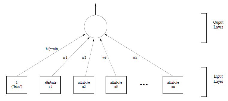
The perceptron (precursor to the neural network) can be pictured as a two layer network (graph) of "neurons" (nodes). The input layer has one node per attribute plus an extra node (the bias, defining the threshold) which is connected to the output node (the only node in the output layer) via a weighted connection. When an instance is presented to the input layer, its attribute values activate the input layer. The input activations are multiplied by weights and then summed. If the weighted sum is greater than 0, then the output signal is 1, otherwise -1.
Version 1 of the Perceptron learning rule is as follows:
Set all weights to 0
Until all instances in the training data are classified correctly:
for each instance I in the training data:
if I is classified incorrectly by the perceptron:
if I belongs to the first class:
add it to the weight vector
else
subtract it from the weight vector
Version 2 of the Perceptron learning rule is:
Given a linearly separable training set S = {a1, ..., an}, learning rate η ∈ R+
w0 ← 0; b0 ← 0; k ← 0
R ← max1≤i≤n||ai||
until no mistakes made within the for loop:
for i = 1 to n:
if xi(⟨wk.ai⟩ + bk) ≤ 0 (i.e., incorrect classification) then:
wk+1 ← wk + ηxiai
bk+1 ← bk + ηxiR2
k ← k + 1
end if
end for
return (wk, bk) where k is the number of mistakes
The perceptron training rule guarantees convergence in a finite number of steps provided the training examples are linearly separable and a sufficiently small η is used.
Support Vector Machines
The main limitation of simple linear classifers is that they can only represent linear class boundaries, making them too simple for many applications. Support vector machines (SVMs) use linear models to implement non-linear class boundaries by transforming input using a non-linear mapping. The instance space is mapped into a new space, and a non-linear class boundary in the original space maps onto a linear boundary in the new space.
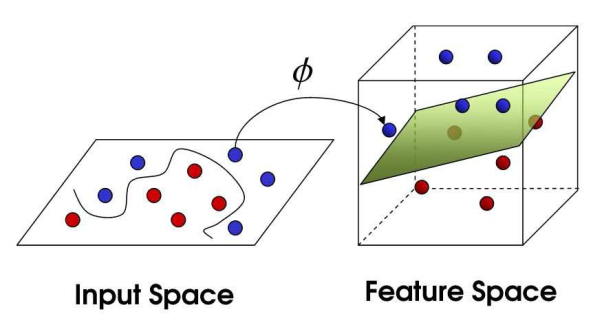
Suppose that we replace the original set of n attributes by a set including all products of k factors that can be constructed from these attributes (i.e., we move from a linear expression in n variables to a multivariate polynomial of degree k). So, if we started with a linear model with two attributes and two weights (x = w1a1 + w2a2), we would move to one with four synthetic attributes and four weights (x = w1a13 + w2a12a2 + w3a12a22 + w4a23).
To generate a linear model in the space spanned by these products of factors, each training instance is mapped into a new space by computing all possible 3 factor products of its two attribute values and the learning algorithm applied to these transformed instances. To classify a test instance, it is transformed prior to classification.
However, there are issues of computational complexity: 5 factors of 10 attributes lead to other 2000 coefficients, and additionally overfitting can occur if the number of coefficents is large relative to the number of training instances (the model is "too nonlinear"). SVMs solve both problems using a linear model called the maximum margin hyperplane.
The maximum margin hyperplane gives the greatest separation between the classes. The perpendicular bisector of the shortest line connecting the convex hulls (tightest enclosing convex polygon) of the sets of points in each class is constructed, and the instances closest to the maximum margin hyperplane are called support vectors, and there is at least one per class. These support vectors uniquely define the maximum margin hyperplane. Given them, we can construct the maximum margin hyperplane and all other instances can be discarded.
SVMs are unlikely to overfit as overfitting is caused by too much flexibility in the decision boundary. The maximum margin hyperplane is relatively stable and only changes if the training instances that are the support vectors are added or removed. Usually, there are few support vectors (which can be thought of as global representatives of the training set) which give little flexibility.
SVMs are not computational infeasible as to classify a test instance, the vector dot product of the test instance with all support vectors must be calculated. The dot product invloves one multiplication and one addition per attribute (expensive in the new high-dimensional space resulting from the non-linear mapping), however we can compute the dot product on the original attribute set before mapping (e.g., if using a high dimensional feature space based on the products of k factors, take the dot product of vectors in low dimensional space and raise the the power k - a function called a polynomial kernel - k usually starts at 1, a linear model, and increased until no reduction in the estimated error).
Other kernel functions can be used to implement different non-linear mappings: radial basis function (RBF) kernel, equivalent to an RBF neural network, or sigmoid kernels, equivalent to a multilayer perceptron with one hidden layer).
The choice of kernel depends on the application and may not be much different in practice. SVMs can be generalised to cases where the training data is not linearly separable, but as slow in training compared to other algorithms, such as decisino trees. However, SVMs can produce very accurate classifiers, and on text classification, the best results are now typically obtained using SVMs.
Artificial Neural Networks
The study of artificual neural networks (ANNs) was inspired by the observation that brains (biological learning systems) are built of complex networks of interconnected neurons.
The human brain is a densely connected network of approximately 1011 neurons, and each neuron is connected, on average, to 104 other neurons. The neuron switching speeds are slow compared to compute speeds, but people can make complex decisions very quickly. This suggests that information processing in neural networks results from highly parallel processing over distributed representations (i.e., representations distributed over many neurons).
ANNs are an approximation of some aspects of biological neural systems. In ANNs, the networks consist of a densely interconnected set of simple units. Each unit takes a number of real-valued inputs (which are possibly outputs of other units) and produces a single real-valued output.
Many of the complexities of biological neural systems are not modelled in ANNs (e.g., artificial neurons single constant values whereas biological neurons output a complex time series of spikes).
Researchers into ANNs tend to fall into two groups - those interested in modelling biological learning processes and those interested in obtaining effective machine learning algorithms, independent of whether or not these reflect actual biological processes.
ANNs are well suited for problems where the training data is noisy, or for complex sensor data. They can also be used for problems involving symbolic representations (e.g., the concept learning problems considered in relation to decision trees).
The most popular ANN learning algorithms - Backpropagation - is suitable for problems where instances are represented by attribute-value pairs, and where the target function output may be discrete-valued, real-valued or a vector of several discrete or real-valued attributed. Backpropagation is also suitable when the training data may contain errors, fast evaluation of the learned target function may be required but long training times are acceptable and a human understanding/representation of the learned target function is not important.
Of key importance is how to learn an ANN. Considerations for such a scheme must consider the design of primitive units that make up the ANN, learning algorithms for training single primitive units and learning algorithms for training multilayer networks.
This module will not consider algorithms for learning network structure (i.e., number of layers and units, and network topology).
Perceptrons (discussed above) are one method by which the primitive units are made up of. Perceptrons can be seen as representing a hyperplane decision surface in n-dimensional instance space. It outputs 1 for instances on one side of the hyperplane and -1 for instances on the other side of the hyperplane.
A single perceptron can represent many boolean functions (e.g., AND), but a single perceptron can not represent all boolean functions (e.g., XOR), however a two-level perceptron network can.
Whilst we eventually want to be able to train networks of multiple interconnected units, we being by studying how to learn weights for a single perceptron - more precisely, we determine a weight vector that causes the perceptron to produce the correct result for each training example.
Several algorithms are known to solve this problem, including the perceptron training rule (discussed above) and the delta rule. Both are guaranteed to converge to somewhat different acceptable hypotheses, under different conditions.
Delta Rule
As the perception training rule is only guaranteed to converge if the training examples are linearly separable. The delta rule is designed to address this difficulty, it converges to a best-fit approximation to a target function if the training examples are not linearly separable.
The key idea behind the delta rule is to use gradient descent to search the hypothesis space of possible weight vectors to find the best fit to the training data. Gradient descent is important because it is the basis of the Backpropagation algorithm (the most popular algorithm for training multilayer ANNs) and can be used as the basis for any learning algorithm that must search a hypothesis space containing hypotheses with continuous parameters.
If we consider the task of training an unthresholded perceptron (i.e., a linear unit) whose output o is given by o(x) = w·x, then we can specify a measure of training error of a hypothesis (weight vector) w.r.t. the training examples: E(w) ≡ 1/2 ∑d∈D(td - od)2, where D is the set of training examples, td is the target output for a training example d and od the output of the linear unit for the training example d.
If we consider a linear unit with just two weights (w0 and w1), then the plane w0,w1 represents the entire hypothesis space. A third dimension exists for the error E for a fixed set of training examples. Given the definition of E, the error surface must always be parabolic with a single global minimum.
Gradient descent search determines a weight vector that minimises E by starting with an arbitrary weight vector, and modifies the vector in small steps by altering it in the direction that produces the steepest descent along the error surface, stopping when the global minimum error is reached.
The derivation of the steepest descent along the error surface is determined by computing the derivative of E w.r.t. each component of the vector w - this is called the gradient of E w.r.t. w. When interpreted as a vector in weight space, the gradient specifies the direction of the steepest increase in E, so the negative of this is the direction of the steepest decrease.
Gradient_Descent(training_examples, η)
Initialise each wi to some small random value
Until the termination condition is met:
initialise each Δwi to 0
for each ⟨x, t⟩ in training_examples:
input the instance x to the unit and compute the output o
for each linear weight wi:
Δwi ← Δwi + η(t - o)xi
for each linear weight wi:
wi ← wi + Δwi
Since the error surface has a single global minimum, this algorithm converges to a weight vector with minimum error regardless of whether the training examples are linearly separable, given a sufficiently small η.
Stochastic Approximation to Gradient Descent
Gradient descent is a general strategy for searching through large/infinite hypothesis spaces (H) whenever H contains continuously parameterised hypothesis, and the error can be differentiated w.r.t. the hypothesis parameters.
Practical difficulties in applying the gradient descent occur as converging to a local minimum can be very slow, and if there are multiple local minima in the error surface, then there is no guarantee the global minimum will be found.
A variant of gradient descent that addresses these issues is called stochastic gradient descent.
The gradient descent computes the weight updates after summing over all the training examples, and the stochastic gradient descent approximates this by updating weights incrementally after the calculation of the error for each example. To achieve this, the second assignment is removed from Gradient_Descent and the first equation replaced with: wi ← wi + η(t - o)xi. This is known as the delta rule.
By making the learning rate η sufficiently small, stochastic gradient descent (SGD) can be made to approximate gradient descent (GD) arbitrarily closely.
The key differences between GD and SGD are that in GD, the error is summed over all the examples before updating weights, whereas in SGD, weights are updated after examning each training example. Additionally, GD requires more computation per weight update step, but because it uses a true gradient, it is often used with a larger step size per weight update than SGD. Also, in cases where there are multiple local minima w.r.t. E(w), SGD can sometimes avoid theses because it is essentially examining the gradient of a distinct error function Ed(w) for each example d, rather than that of the single error function E(w).
The delta rule converges asymptopically toward the minimum error hypothesis, possibly requiring unbounded time, regardless of whether the training examples are linearly separable.
Multilayer Networks
Single perceptrons can only express linear decision surfaces. Interesting real world problems often involve learning decision boundaries. Multiple layers of cascaded linear units still only produce linear functions, so they are not appropriate if we want to learn non-linear functions. Perceptrons are another possiblity, but discontinuous thresholds means it is undifferentiatable and hence not suitable for gradient descent.
One solution is the sigmoid unit - like a perceptron, but based on a smoothed, differentiable threshold function. The sigmoid's output o is given by o = σ(w·x) where σ(y) = 1/(1 + e-y).
Backpropagation Algorithm
The Backpropagation algorithm learns the weights for a multilayer network governing a network with a fixed set of units and connections. It uses gradient descent to try and minimise the squared error between the network outputs and the target values for the same inputs that produced these outputs.
Since we are dealing with a network with multiple output units, rather than one as before, E must be redefined to sum the error over all the output units: E(w) ≡ 1/2 ∑d ∈ D∑k∈outputs(tkd - okd)2, where outputs is the set of output units, tkd and okd are the target and output valyes of the kth output unit for the training example d.
The learning problem is to search a hypothesis space defined by all possible weight values for all units in the network. This can be visualised in terms of an error surface as before, except now the error is defined as above and one dimensional in the space needed for each of the weights associated with the units in the network. As before, we can now use gradient descent to search for a hypothesis to minimise E.
The algorithm is outlined on
slide 24 of lecture 18.
In multilayer networks, the error surface may have multiple local minima, and backpropagation is only guaranteed to converge toward some local minimum, not the global minimum error. Despite this, it has been remarkably successful in practice.
The algorithm as stated only applied to two level feedforward networks, but can be straightforwardly extended to feedforward networks of any depth.
The gradient descent weight update rule is similar to the delta rule. Like the delta rule, each weight is updated in proportion to the learning rate η, the input value xji to which the weight is applied and the error in the output of the uni, but the error (t - o) in the delta rule is replaced by the more complex error term δj. The exact form of δj follows from the mathematical derivation of the backpropagation weight tuning rule.
The backpropagation algorithm presented corresponds to stochastic gradient descent.
Association Rule Mining and Clustering
So far we have primarily focussed on classification, which works well if we understand which attributes are likely to predict others and/or we have a clear-cut classification in mind, however in other cases there may be no distinguished class attributes.
We may want to learn association rules capturing regularities underlying a dataset. Given a set of training examples represented as pairs of attribute-value vectors, then learn if-then rules expressing significant associations between attributes.
We may also want to discover clusters in our data, either to understand the data or to train classifiers. Given a set of training examples, and some measure of similarity, we want to learn a set of clusters caputing significant groupings amongst the instances.
Association Rule Mining
We could use the rule learning methods studied earlier, considering each possible combination of attributes as a possible consequent of the if-then rule and then prune the resulting association rules by coverage (or support - the number of instances the rules correctly predict) and accuracy (or confidence - the proportion of instances to which the rule applies which it correctly predicts). However, given the combinatorics, such an approach is computationally infeasible. Instead, we base the approach on the assumption that we are only interested in rules with some minimum coverage. We look for combinations of attribute-value pairs with pre-specificed minimum coverage, called item sets - where an item is an attribute-value pair.
We start by sequentially generating all 1-item, 2-item, ..., n-item sets that have minimum coverage. This can be done efficiently by observing that an n-item set can achieve minimum coverage only if all of them n - 1-item sets which are subsets of the n-item set have minimum coverage.
Next, we form rules by considering for each minimum coverage item set all possible rules containing 0 or more attribute-value pairs from the item set in the antecedent and one or more attribute-value pairs from the item set in the consequent. The coverage for each rule is then computed: number for which the consequent is correct / number for which the antecedent matches.
Clustering
Approaches to clustering can be characterised in various ways. One such characterisation is by the type of clusters produced.
Clusters may be partitions of the instance space (each instance is assigned to exactly one cluster), overlapping subsets of the instance space (instances may belong to more than one cluster), probabilities of cluster membership are associated with each instance, and hierarchial structures, e.g., tree-like dendograms (any given cluster may consist of subclusters, or instances, or both).
Hierarchial clustering can be: agglomerative (bottom-up), which starts with individual instances and then groups the most similar; divisive (top-down), which starts with all instances in a single cluster and divides them into groups so as to maximise within group similarity; and mixed, which starts with individual instances and either adds to an existing cluster or forms a new cluster, possibly merging or splitting instances in existing clusters (e.g., CobWeb).
Non-hierarchial (flat) clustering can take either: a partitioning approach where k clusters are hypothesised, and then cluster centres are randomly picked, and instances are iteratively assigned to the centres, and the centres recomputed until stable, and; probabilistiv approaches, which hypothesises k clusters each with an associated (initially gussed) probability distribution of attribute valyes for instances in the cluster, then the cluster probabilities for each instance are iteratively computed, and the cluster parameters recomputed until stability.
Another taxonomic attribute to consider is incremental vs. batch clustering - are clusters computed dynamically as instances become available, or statically on the presumption that the whole instance set is available?
Agglomerative Clustering
Given a set X = {x1, ..., xn} of instances and a function sim: 2X × 2X → R
for i = 1 to n:
ci ← {xi}
C ← {c1, ..., cn}
j ← n + 1
while |C| > 1:
(cn1, cn2) ← argmax(cu, cv)∈C×C(cu, cv)
cj ← cn1 ∪ cn2
C ← C \ {cn1, cn2} ∪ {cj}
j ← j + 1
return C
Essentially, we start with a separate cluster for each instance and then repeatedly determine the two most similar clusters and merge them together. We terminate when a single cluster containing all instances has been formed.
Divisive Clustering
Given a set X = {x1, ..., xn} of instances + a function coh: 2X → R + a function split: 2X → 2X × 2X
C ← {X} (= {c1})
j ← 1
while &exists;ci ∈ C such that |ci| > 1:
cu ← argmincv∈Ccoh(cv)
(cj+1,cj+2) = split(cu)
C ← C \ {cu} ∪ {cj+1, cj+2}
j → j + 2
return C
Essentially, we once again start with a single cluster containing all instances, and then repeatdely determine the least coherent cluster and split it into two subclusters. We terminate when no cluster comtanis more than one instance.
Similarity Functions
The single link function is when the similarity between two clusters = similarity of the most similar members, the complete link = similarity of the two least similar members and the group average = average similarity between members.
Single link clustering results in elongated clusters (chaining effect) that are locally coherent in that close objects are in the same cluster, but may have poor global quality.
Complete link clustering avoids this problem by focussing on global rather than local quality - this reuslts in "tighter" clusters. Unfortunately complete link clustering has time complexity O(n3), compared to single link clusterings O(n2).
Group average clustering is a compromise that is O(n2), but avoids the elongated clusters of single link clustering. The average similarity between vectors in a cluster c is defined as S(c) = 1/(|c(|c| - 1))∑x∈c∑x≠y∈csim(x,y).
At each iteration, the clustering algorithm picks two clusters cu and cv that maximises S(cu ∪ cv). To carry out group average clustering efficiently, care must be taken to avoid recomputing average similarities from scratch after each of the merging steps. We can avoid donig this by representing instances are length-normalised vectors in m-dimensional real-valued space and using the cosine similarity measure. Given this approach, the average similarity of a cluster can be computed in constant time from the average similarity of its two children.
In top down hierarchial clustering, a measure is needed for cluster coherence and an operation to split clusters must be defined. The similarity measures already defined for bottom-up clustering can be used for these tasks.
Coherence can be defined as: the smallest similarity in the minimum spanning tree for the cluster (the tree connecting all instances the sum of whose edge lengths is minmal) according to the single link similarity measure; the smallest similarity between any two instances in the cluster, according to the complete link measure, or; the average similarity between objects in the, according to the group average measure.
Once the least coherent cluster is identified, it needs to be split. Splitting can be seen as a clustering task - find two subclusters of a given cluster - and any clustering algorithm can be used for this task.
Non-hierarchial Clustering
Non-hierarchial clustering algorithms typically start with a partition based on randomly selected seeds and then iteratively refines this partition by reallocating instances to the current best cluster (in contrast with hierarchial algorithms which typically require only one pass).
Termination occurs when, according to some measure of goodness, clusters are no longer improving. Measures include group average similarity, mutual information between adjacent clusters, and the likelihood of data given the clustering model.
The number of clusters can be determined perhaps by some prior knowledge, or by trying various cluster numbers, n, and seeing how the measures of goodness compare, or if there is a reduction in the rate of increase of goodness for some n. Also, minimum description length can be used to minimise the sum of the lengths of encodings of instances in terms of distance from clusters and the encodings of clusters.
Hierarchial clustering does not require a number of clusters to be determined, however full hierarchial clusterings are rarely usable and the tree must be cut at some point, which is equivalent to specifying a number of clusters.
k-means Clustering
Given a set X = {x1, ..., xn} ∈ Rm, and a distance measure d : Rm × Rm → R, and a function for computing the mean μ : P(R) → Rm
select k initial centres f1, ..., fk
while the stopping criterion is not true:
for all clusters cj:
cj = {xi | ∀f1d(xi, fi) ≤ d(xi, fi)}
for all means fi:
fi = μ(cj).
This algorithm picks k initial centres and forms clusters by allocating each instance to its nearest centre. Centres for each cluster are recomputed as the centroid, or mean, of the cluster's members μ = (1/|cj)∑x∈cjx and instances are once again allocated to their nearest centre. The algorithm iterates until stability or some other measure of goodness is attained.
Probability-based Clustering and the EM algorithm
In probability-based cluster, an instance is not placed categorically in a single cluster, but rather is assigned a probability of beloning to every cluster.
The basis of statistical clustering is the finite mixture model - a mixture of k probability distributeion representing k clusters. Each distribution gives a probability that an instance would have a certain set of attribute values if it were known to be a member of that cluster.
The clustering problem is to take a set of instances and a pre-specified number of clusters and work out each cluster's mean and variance, and the population distribution between clusters. Expectation-Maximisation (EM) is an algorithm for doing this.
Like k-means, we start with a guess for the parameters governing clusters. These parameters are used to calculate cluster probabilites for each instance (the expectation of class values), and these probabilities used for each instance to re-estimate cluster parameters (maximisation of the likelihood of the distributions given the data). We then terminate when some goodness measure is met - usually when the increase in log likelihood that the data came from the finite mixture model is negligible between iterations.
Combining Multiple Models
People making critical decisions usually consult several experts. A model generated by an ML technique over some training data can be viewed as an expert, so it is natural to ask whether or not we can combined judgements of multiple models to get a decision that is more reliable than of any single model. We can, but not always and the resulting combined models may be hard to understand or analyse.
If we suppose (ideally) that we have an infinite number of independent training sets of the same size from which we train an infinite number of classifiers (using one learning scheme) which are used to classify a test instance via majority vote, then such a combined classifier will still make errors, depending on how well the machine learning method fits the problem, and the noise in the data.
If we were to average the error rate of the combined classifer across an infinite number of independently chosen test examples, we arrive at the bias of the learning algorithm for the learning problem. This is the residual error that can not be eliminated regardless of the number of training sets. A second source of error arises from the use, in practice, of finite datasets, which are inevitably not fully representative of the entire instance population. The average of this error over all training sets of a given size, and all test sets, is the variance of the learning method for this problem.
The total error is the sum of the bias and the variance (bias-variance decomposition) and combining classifiers reduces the variances component of the error.
Bagging
Bootstrap aggregating ("Bagging") is a process whereby a single classifier is constructed from a number of classifiers. Each classifier is learned by applying a single learning scheme to multiple artificial training datasets that are derived from a single, original, training dataset.
These artificial datasets are obtained by randomly sampling with replacement from the original dataset, creating new datasets of the same size. The sampling procedure deletes some instances and replicates others.
The combined classifier works by applying each of the learned classifiers to novel instances, and deciding their classification by majority vote. For numeric predictions, the final values are determined by averaging the classifier outputs.
Bagging produces a combined model that often performs significantly better than a single model built from the original data set, and never performs substantially worse.
Randomisation
Bagging generates an ensemble of classifiers by introducing randomess into the learner's input. Some learning algorithms have randomless built-in. For example, perceptrons start out with randomly assigned connection weights that are then adjusted during training. One way to make such algorithms more stable is to run them several times with different random number seeds and combine the classifier predictions by voting or averaging.
A random element can be added into most learning algorithms.
Randomisation requires more work than bagging, because the learning algorithm has to be modified, however it can be applied to a wider range of learners; bagging fails with stable learners (those whose output is insensitive to small changes in input), however randomisation can be applied by, e.g., selecting differently randomly chosen subsets of attributes on which to base the classifiers.
Boosting
Like bagging, boosting works by combining (via voting or averaging), multiple models produced by a single learning scheme. Unlike bagging, it does not derive models from artificially produced datasets generated by random sampling, instead if builds models iteratively, with each model taking into account the performance of the last.
Boosting encourages subsequent models to emphasise examples badly handled by earlier ones. This builds classifiers whose strengths complement each other.
In AdaBoost.M1, this is achieved by using the notion of a weighted instance. The error is computed by taking into account the weights of misclassified instances, rather than just the performance of the misclassified instances. By increasing the weight of misclassified instances following the training of one model, the next model can be made to attend to these instances. The final classification is determined by weighted voting across all the classifiers, where weighting is based on classifier performance (in the AdaBoost.M1 case by the error of the individual classifiers).
AdaBoost.M1
Model Generation:
Assign equal weight to each training instance:
For each of t iterations:
apply the learning algorithm to the weighted dataset and store the resulting model
nbsp; compute the error e of the model on the weighted dataset and stored the error
if e = 0 or e ≥ 0.5:
then terminate model generation
for each instance i in the dataset:
if i classified correctly by model:
then weighti ← weighti × e/(1 - e)
Normalise the weight of all instances so that their summed weight remains constant.
Classification:
Assign weight of 0 to all classed
For each of the t (or less) models:
Add -log(e/(1 - e)) to the weight of each class predicted by the model
return the class with the highest weight.
Boosting often performs substantially better than bagging, but unlike bagging, which never performs substantially worse than a single classifier built on the same data, boosting sometimes can do (overfitting).
Interestingly, performing more boosting iterations after the error on the training data has dropped to can further improve performance on new test data. This seems to contract Occam's razor (preference of simpler hypothesis), since more iterations lead to more complex hypothesis which does not explain the training data better, however, more interations improve the classifier's confidence in its predictions - the difference between the estimated probability of the true class and that of the most likely predicted class other than the true class (called the margin).
Boosting allows powerful combined classifier to be built from simple ones (provided they achieve < 50% error rate on reweighted data). Such simple learners are called weak learners and include decision stumps (one level decision trees) or OneR.
Stacking
Bagging and boosting combine multiple models produced by one learning scheme. Stacking is normally used to combine models built by different learning algorithms. Rather than simply voting, stacking attempts to learn which are the reliable classifiers using a metalearner.
Inputs to the metalearner are instances built on the outputs of level 0, or base level, models. These level 1 instances consist of one attribute for each level 0 learner - the class the level 0 learner predicts for the level 1 instance. For these instances, the level 1 model makes the final prediction.
During training, the level 1 model is given instances which are the level 0 predictions for the level 0 instances, plus the actual class of the instance. However, if the predictions of the level 0 learners over the data they were trained on are used, the result will be a metalearner trained to prefer classifiers that overfit the training data.
In order to avoid overfitting, the level 1 instances must either be formed from level 0 predictions over instances that were held out from level 0 training, or from predictions on the instances in the test folds, if cross-validation was used for training at level 0.
Stacking can be extended to deal with level 0 classifiers that produce probability distributions over output class labels, and numeric prediction rather than classification.
Whilst any ML algorithm can be used at level 1, simple level 1 algorithms such as linear regression have proved best.
Using Unlabeled Data
Labeled training data (i.e., data with the associated target class) is always limited and frequently requires an extensive/expensive manual annotation or cleaning process. However, large amount of unlabeled data may be readily available. We can consider utilising unlabeled data to improve a classifier.
Clustering
One possibility is to couple a probabilistic classifier (such as naive Bayes) with Expectation-Maximisation (EM) iterative probabilistic clustering. If we suppose we have some labelled training data L and some unlabelled training data U, then we proceed as follows:
Train naive Bayes on L
repeat until convergence:
(E-step) use the current classifier to estimate the component mixture for each instance (i.e., the probability that each mixture component generated each instance)
(M-step) re-estimate the classifier using the estimated component mixture for each instance in L + U
output a classifier that predicts labels for unlabelled instances.
Experiments show that such a learner can attain equivalent performance to a traditional learner using < 1/3 the labeled training examples together with 5 times as many unlabled examples.
Co-training
Suppose that there are two independent perspectives or views (feature sets) on a classification task, then co-training exploits these two perspectives.
We train model A using perspective 1 on the labeled data, and then model B using perspective 2 on the data. The unlabeled data is using labeled using models A and B separately. For each model, we select the example it most confidently labels positively, and the one is most confidently labels negatively, and add these to the pool of labeled examples. This process is then repeated on the augmented pool of labeled examples until there are no more unlabeled examples.
There is some experimental evidence to indicate co-training using naive Bayes as a learner outperforms an approach which learns a single model using all features from both perspectives.
Co-EM
Co-EM trains model A using perspective 1 on the labeled data, and then uses model A to probabilistically label all the unlabeled data. Model B is then trained using perspective 2 on the original labeled data, and the unlabeled data tentatively labeled using model A. Model B is then used to probabilistically relabel all the data for use in retraining model A. This process then iterates until the classifiers converge.
Co-EM appears to perform consistently better than co-training (because it does not commit to class labels, but re-estimates their probabilities at each iteration).
Both co-training and co-EM are limited to applications where multiple perspectives on the data are available. Some recent evidence suggests that this split can be artificially manufactured (e.g., using some random selection of features, though feature independence is preferred) and some recent arguments and evidence that co-training using models derived by different classifiers (instead of from different feature sets) also works.