Computer Science notes ⇒ COM6791: Natural Language Processing

To fully describe a language, we must consider the sounds which make up each word, the order in which the words occur, the meaning of these words and the types of situations in which a sentence can be uttered.

Linguists typically make the assumption that language can be described on a number of levels, and that these levels can largely be studied independently. There is no full agreement as to what these levels are, or how they are related, but the generally agreed levels of descriptions are: phonetics, phonology, graphetics, graphology, morphology, syntax, semantics, discourse and pragmatics.

Phonetics is the study of how to describe and classify speech sounds - typically using some articulatory description (e.g., referring to how the sounds are produced in the human vocal tract). Phonetics is independent of the language of the speaker, concerned with the total range of vocal sounds humans can produce and detect. Phonology is the study of the principles that govern which sounds are used in actual human languages, and explaining those patterns and variations. Phonology seeks to find minimal sound units, called phonemes, which, if changed in a word, alter the word's meaning.

By analogy to phonetics and phonology, graphetics is the study of the physical properties of the symbols making up writing systems, including study of the means of production of symbols, and graphology is the study of the characteristics of the symbol system used in human languages. Graphemes, analogous with phonemes, are the smallest unit in the writing system whose change affects meaning, e.g., c and c are the same grapheme.

Although there are physical faculties associated with spoken language (Broca's area - a region of the brain shown to be linked to language, and vocal apparatus) appear to have arisen in homo sapiens over 300,000 years ago, written language only emerged more recently, about 5000 years ago. There is some dispute whether earlier evidence of writing forms a writing system. Some people define a writing system as "a system of more or less permanent marks used to represent an utterance in such a way that it can be recovered more or less exactly with the intervention of the utterer".

Writing systems can be classified as logographic, where symbols represent words (e.g., Hanzi or Kanji); syllabic, where symbols represent syllables; and alphabetic, where symbols represent phonemes. Alphabetic systems can be broken up into abugidas, which are syllabic, but diacritics or other modifications are used to indicate which vowels is used; abjads, which are consonants only and the speaker inserts an appropriate vowel, which diacritics used to indicate non-standard vowels, and alphabets.

Morphology is the study of the structure of words. The smallest meaningful elements into which words can be decomposed are called morphemes. Morphology is typically divided into the two subfields of inflections and derivational morphology.

Inflectional morphology is concerned with the differing forms one words takes to signal differing grammatical roles (e.g., boy (singular) vs. boys (plural)); inflected forms are of the same syntactic category. Derivational morphology is concerned with how new words may be constructed from component morphemes (e.g., institute to institution to institutional, etc).

Syntax is the study of the structure of sentences, however this is no consensus on the definition of a sentence. For NLP, we proceed by analysing linguistic constructions that actually occur and identifying those that can stand on their own and possess syntactic structure. Traditionally, a hierarchy of sentence structure is recognised: sentence → clauses → phrases → words → morphemes. Like sentence, neither the terms clause nor phrase are precisely defined, but are useful in talking about sentences.

Sentence structure is frequently displayed graphically by means of a phrase structure tree. The words of the sentence label the tree's leaves, whilst non-lead nodes are labelled with grammatical categories (e.g., NP/VP). An alternative representation is labelled bracketing.

A catalogue of structural descriptions purporting to describe the sentence structure of a language is called a grammar - these structural descriptions are called grammar rules. It is important to differentiate between prescriptive vs. descriptive grammar rules.

Semantics is the study of the meaning in language. The study of the definition of meaning has preoccuped generations of philosophers. The ultimate question of meaning can be set aside for NLP, but it is essential to derive a representation of a text that can be manipulated to achieve some goal.

Discourse analysis involves the analysis of the structure and meaning of discourse or text (i.e., of multiple sentence linguistic phenomena). Some topics of study include that of textual structure, such as coreference (knowing if two different linguistic expressions refer to the same thing), ellipsis (structure which may be omitted and recovered from the surrounding text) and coherence (what it is that makes multi-sentence texts coherent, e.g., rhetorical structure theory - a set of relationships between sentences or clauses). Other topics of study include that of conversational structure, e.g., signalling ends of conversational turns or desire to take one, and of conversational maxims.

Pragmatics is the study of how humans use language in social settings to achieve goals, such as speech acts (promising, resigning, etc) and conversational implicature (not directly responding, but implying an answer). Pragmatics are a subject area is not well-defined, and there is much overlap with discourse analysis.

Computational linguistics has developed models to address all of these aspects of language.

The exact tokenisation rules that should be carried out is dependent on the orthographic conventions adopted in the writing system or script being processed. A script is the system of graphical marks employed to record the expressions of a language in a visible form.

There is a many-to-many mapping between languages and scripts, as many languages may share one script (e.g., Western European languages onto Latin script), and some languages may have multiple scripts (e.g., Japanese's kanji and hiragana).

Scripts may be classified along a number of dimensions: directionality (e.g., left-to-right, right-to-left, etc); historical derivation; and the relationship between the symbols and sounds. The latter is the most common way to classify scripts, but there is no consensus as to subclassifications.

Non-phonological scripts can be:

• pictographic, where the graphemes (called pictographs or pictograms) provide recognisable pictures of entities in the world;
• ideographic, where the graphemes (called ideographs or ideograms) no longer directly represent things in the world, but have an abstract or conventional meaning, and may contain linguistic or phonological elements;
• hieroglypic, which contains ideograms and phonograms to create a rebus where the ideogram for a world is made up of phonograms for the consonants in the word (e.g., "bee" + "r" = "beer") and determinatives to disambiguate between multiple senses;
• logographic, where the graphemes (called logographs or logograms) represent words or part of words. Some characters derive from earlier ideograms, whereas others are phonetic elements, or modified version of base characters to indicate words of related meaning.

Phonological scripts can be:

• syllabic - where graphemes correspond to spoken syllables, typically a vowel-consonant pair;
• alphabetic - where there is a direct correspondence between the graphemes and phonemes of the language. An ideal situation would be a one-to-one grapheme-phoneme mapping, but this is uncommon in natural language as the written form often does not keep pace with pronunciation.

A character, or grapheme, is the smallest components of a written language that has a semantic value. A glyph is a representation of a character or character as they are rendered or displayed. A repertoire of glyphs makes up a font.

The relationship between glyphs and characters can be complex, as for any character, there may be many glyphs (different fonts) representing it, and sometimes single glyphs may correspond to a number of characters, and perhaps a degree of arbitrariness, especially with diacritics.

The goal of morphological parsing is to take a given surface word form and to analyse it discover the stem and any morphological feature information conveyed by any affixes. This morphological feature information can include the part-of-speech, the number (e.g., singular, plural, etc) or the verb form.

The goal of morphological generation is to take a given word stem and some morphological feature information, and from this generate a surface word form.

To do morphological parsing and generation, we need: a lexicon consisting of a list of stems and affixes and additional information, such as whether the stem is a verb or noun stem; morphotactics, which are a model of morpheme ordering that explains which classes of morphemes follow which other classes; and orthographic rules, which are spelling rules that model changes in a word, typically at morpheme boundaries.

FSTs provide an effective computational framework in which to build morphological parsers/generators.

If we assume that the associated information in the lexicon includes morphotactic informatino such as whether a noun is regular, irregular singular or plural, we can build a FSA like so:

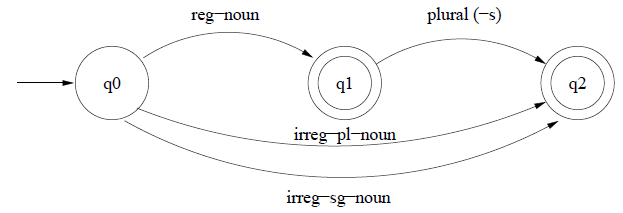
More example FSAs are on
slide 14 onwards of lecture 4

These morphotactic FSAs can be combined with relevant sub-lexicons, expanding arcs like reg-noun with all the morphemes that make up a class to build morphological recognisers - programs that recognise strings that make up legitimate English words.

However, we don't want to just recognise surface forms, we want to parse them yielding stem and morphological features. Thsi can be done using an FST, which views parsing and generation as a bi-directional mapping between the lexical level, representing the concatenation of morphemes (stem + morphological features) and the surface level (the final spelling of the word). This two-level morphology model was first proposed by Koskenniemi in 1983.

We can think of an FST that maps between strings on a two-tape automaton, or as a two-tape automaton that recognises pairs of strings.

In the two-level morphology model, the input symbol on an FST arc corresponds to a character on the lexical level, and the output symbol to a character on the surface level. Symbols commonly map to themselves directly, e.g., a:a, and these are called default pairs, and often compressed down to just the single letter "a".

The FSAs and lexicons discussed above for morphological recognition can be extended for parsing by converting the morphotactic FSAs to FSTs by adding a lexical level tape and morphological features, and by allowing the lexical entries to have two levels. We often include ε here, as well as the special symbols ^ to indicate a morpheme-boundary and # to be the word-boundary. Additionally, @ is a wildcard symbol, with @:@ meaning "any feasible pair", allowing any possible suffixes.

However we also need to consider orthographic rules where regular nouns undergo spelling changes at morpheme boundaries. We can model these rules by using FSTs that work on the output of the two-level model, treating it as including the morpheme boundary symbols as an intermediate level.

We can use rule formalisms such as a → b / c__d, which means "rewrite a as b when it occurs between c and d. For example, the rule for e-insertion may be: ε → e / [xsz]^__s#.

This yields a three level model: the lexical level (stem + morphological information, e.g., fox +N +PL), the intermediate level (including boundary information, e.g., fox^s#) and the surface level (the final word, e.g., foxes).

The lexical FSTs can be combined with the orthographic rule FSTs to create a single parsing/generation system. These FSTs can be cascaded or combined into a single machine using composition and intersection operations.

If we suppose that we pause at a given word in a sentence, we can say that although it is impossible to know exactly which word will follow, we can say that some are more likely than others. Word sequence models allow us to assign probabilities to which words are likely to follow others in a sentence.

These type of models are useful for speech recognition (deriving word sequences from phone sequences), augmentative communication systems, context-sensitive spelling correction, and word completion in limited input devices such as mobile phone keypads.

Probabilistic models are based on counting things. We therefore need to decide what to count, and where to find the things to count. Statistical models of language are built from corpora (many corpus), which are collections of digital texts and/or speech. Many corpora exist, and which corpus is used to train a model has a significant impact on the nature and potential use of the model.

There are a number of issues we need to be clear on. Similar to tokenisation, one is the definition of word, specifically, whether or not punctuation characters count as words in the model.

In the transcriptions of spoken language, word fragments and pause markers occur, and it is often application dependent on whether or not these are counted.

Another consideration is that of wordforms vs. words (e.g., is families and family the same word?), and similar with case-sensitivity (e.g., at the start of sentences, or proper nouns). Most statistical modelling approaches counts wordforms (i.e., inflected forms as they occur in the corpus are counted separately).

We want to be able to derive a probabilistic model that will allow us to compute the probability of entire word sequences (e.g., sentences), or the probability of the next word in a sequence.

If we suppose that any word is equally likely to appear at any point in a text, then for a vocabulary V of size |V|, the probability of a wordform following any other wordform is 1/|V|.

Of course, words are not equally likely to appear at any point, however we could make this model slightly more sophisticated by assuming words occur with the probability that reflects their frequency of occurence across the corpus - this is called the unigram probability.

Rather than looking at the relative frequencies of individual words, we should look at the conditional probabilities of words given their preceding words (e.g., the probability of "the" is much lower immediately following another "the" than otherwise).

If we suppose a word sequence of n words is represented such that w₁...w_n, or wⁿ₁ and consider each word occurring in its correct position as an independent event, the probability of the sequence can be represented as: P(w₁, w₂, ..., w_n), which can be decomposed to ∏ⁿ_k=1P(w_k|w_k-11) using the chain rule.

However, computing P(w_n|w^n-1₁) requires a fantastically large corpus when n>4 - data sparsity problem. The solution here is to make the Markov assumption, which approximates the probability of the nth word in a sequence given n-1 preceding words by the probability of the nth word given a limited number k of preceding words.

The general equation for N-gram approximation to the conditional probability of the next word in a sequence is P(w_n|wⁿ₁) ≈ P(w_n|w^n-1_n-N+1)

Setting k=1 yields a bigram model, and k-2 a trigram model. If we take the bigram case and substitute the approximation into the equation for computing sentence probability for n words, we get: P(wⁿ₁) ≈ P(w_k|w_k-1)

To train a bigram model using a corpus, we need for each bigram to count the number of times it occurs, and then divide it by the number of bigrams that share the first word, or the number of times the first word in the bigram occurs.

For N-grams of any length, the more general form can be used: P(w_n|w^n-1_n-N+1) = C(w^n-1_n-N+1 w_n)/C(w^n-1_n-N+1 w_n)

This approach estimates the N-gram probability by dividing the observed frequency of a sequence by the observed frequency of its prefix - this ratio is called a relative frequency. Using relative frequencies to estimate probabilities is one example of Maximum Likelihood Estimation (MLE). The resulting parameter estimates maximise the likelihood of the corpus C, given the model M (i.e., maximises P(C|M)).

Computing the products of bigram probabilities in a sentence frequently results in underflow. One solution is to take the log of each probability (the logprob), which can then be summed and the anti-log taken.

One issue with the bigram approach is that of data sparsity, where certain plausible bigrams do not occur within our training corpus, giving a probability for a particular bigram, and subsequently of the entire sentence, of 0. As something that has not yet been observed does not necessarily have a probability of 0, we need some way of estimating low probability events that does not assign them 0 probability.

Smoothing is one method to overcome 0 occurrence bigrams. These approaches work by assigning some probability to bigrams unseen in the training data, sometimes including those who are seen very few times (and therefore have unreliable estimates). In this case, we must also reduce the probabilities of seen bigrams so that the total probability mass remains constant.

Add-one Smoothing

Good-Turing Discounting

In interpolation approaches, the probability estimates from all order n-grams are always mixed, e.g., in the trigram case, a weighted interpoliation of trigram, bigram and unigram counts are used.

In simple linear interpolation, we estimate P(w_n|w_n-1, w_n-2) by mixing unigram, bigram and trigram estimates, each weighted by a constant λ such that ∑_iλ_i=1: P(w_n|w_n-1, w_n-2) = λ₁P(w_n|w_n-1, w_n-2) + λ₂P(w_n|w_n-1) + λ₃P(w_n).

More sophisticated versions allow the λ weightings to be conditioned on context, for example, if we have particularly trustworthy trigrams, we can weight such trigrams more to get better results.

For both simple and conditional interpolation approaches, the λs must be determined. This is done using a held-out corpus, one different from the training corpus. The training corpus is used to acquire the n-gram counts and fix n-gram probabilities, then the values for λs that maximise the likelihood of the held-out corpus. A machine learning algorithm such as Expectation Maximisation (EM) can be used to learn this.

Simple linear interpolation is easy to understand and implement, but there are better models, such as backoff with Good-Turing discounting, called Katz backoff.

In backoff approaches, n-gram counts are used exclusively if n-gram counts are non-zero, and we only back-off to lower order n-grams if no evidence exists for the higher-order n-gram.

Slide 7, lecture 7 has
contains the general form of
probability estimates.

Discounting, which provides a way to assign probabilities to unseen events, is an integral part of the algorithm. In earlier discussions of Good-Turing, we assumed that all unseen events are equally probable and distributed probability mass available from discounting equally among them. In Katz backoff, Good-Turing discounting is used to calculate the total probability mass for unseen events, and backoff is used to determine how to distribute this amongst unseen events.

Discounted probabilities P* and weights α must be used, otherwise the results of these equations are not true probabilities (that is, where the sum of all probabilities = 1). P* is used to compute the amount of probability mass to save for lower order n-grams, and the α is used to ensure the amount of probability mass contributed by the lower-order model sums to the amount saved by discounting higher order N-grams.

The closed vocabulary assumption is the assumption that we know the vocabulary size V in advance. Language models are then trained and tested on corpora containing only words from the closed vocabulary.

This assumption is unrealistic, as real world text always contains previously unseen words (new proper names, neologisms, new terminology, etc). These previously unseen words are called unknown, or out-of-vocabulary (OOV) words. The percentage of OOV words in a test set is the OOV rate.

Generally, an open vocabulary system is more desirable, as it can handle OOV words. A typical approach to model such unknown words in the test set is by adding a pseudo-word "UNK" to the vocabulary, and training the probabilities to model it by fixing a vocabulary in advance, and converting an OOV word in the training set to UNK prior to training. The counts for UNK can then be estimated just as for any other word in the training data.

The best way to evaluate an n-gram language model is to embed the model in an application (e.g., a speech recogniser) and see if it makes a difference. However, such evaluation can be difficult.

An alternate, more direct, measure is perplexity. Although an improvement in perplexity does not guarantee improvements in applications, it is often correlated with such improvements.

The intuition underlying perplexity as an evaluation measure is that it is a measure of how well a model fits some test data. This measure of fit is the probability of the test data, given some model, and the model that better fits the data is the one that assigns it a higher probability.

For a test set W = w₁w₂...w_n, perplexity (PP) is formally defined as the probability of the test set, normalised by the number of words: PP(W) = P(w₁w₂...w_n)^-1/N

If we make our conditional independence assumption and use the bigram case, then the chain rule of probability allows us to expand this to: PP(W) = ^N√∏^N_i=11/P(w_i|w_i-1)

Note that perplexity is inversely related to the conditional probability of the word sequence (i.e., minimising perplexity maximises the test set probability, according to the language model). In evaluating a language model, it is usual to use the entire word sequence of some test corpus.

Another way to think of perplexity is as the average weighted branching factor (the number of possible next words for a given word) of a language. Where the branching factor is where each word following is equally likely, the weighted branching factor is the one which takes into account the likeliness of the following word.

When computing the perplexity, it is important that the test set is distinct from the training set, as knowledge of the test set (e.g., of the vocabulary) can artificially lower the perplexity.

Perplexity can also be defined in terms of cross-entropy. If we recall that entropy of a random variable X over a set χ (e.g., letters or words) is defined by: H(X) = -∑_x∈χp(x)log₂p(x), where p(x) = P(X=x).

However, we are interested in computing the entropy of finite word sequences of a language L, so our X is a word sequence, and χ the language. From this, we can define the entropy rate, or per-word entropy: 1/nH(Wⁿ₁) = -1/n ∑_{Wⁿ1 ∈ L} p(Wⁿ₁) log₂p(Wⁿ₁)

To measure true entropy of a language, we need to think about sequences of infinite length. If we consider language as a stochastic process, L, that generates a sequence of words: H(L) = lim_n→∞ 1/n ∑_W∈Lp(w₁, w₂, ..., w_n)log p(w₁, w₂, ..., w_n)

Shannon-McMillan-Breiman Theorem states that if the language is regular (stationary and ergodic): H(L) = lim_n→∞ -1/n log p(w₁, w₂, ..., w_n), i.e., take a single sequence that is long enough instead of summing over all possible sequences. Intuition is that a long enough sequence of words will contain in it many other shorter sequences, and that each of these shorter sequences will reoccur in the longer sequence according to their probabilities.

Cross-entropy is useful when we don't know the true probability distribution p that generated some data, but do have a model m that approximates it. For a distribution p, and our attempt to model it, m, the cross entropy of m on p is defined as: H(p, m) = lim_n→∞ 1/n ∑_W∈Lp(w₁, w₂, ..., w_n)log m(w₁, w₂, ..., w_n), i.e., we draw sequences according to p, but sum the log of their probabilities according to m.

If we apply the Shannon-McMillan-Breiman theorem for stationary ergodic processes: H(p, m) = lim_n→∞ -1/n log m(w₁, w₂, ..., w_n) removes the dependency on the unknown true dependency p.

For any model m, H(p) ≤ H(p, m), i.e., cross-entropy is an upper bound on entropy. The better m is, the closer the cross-entropy is to the true entropy H(p), so cross-entropy can be used to compare two models, and the better model is the one with the lower cross-entropy.

We can approximate the cross-entropy for a model M = P(W) trained over a sufficiently long fixed length sequence W by H(W) = -1/N log P(w₁, w₂, ..., w_n).

The perplexity of a model P on a word sequence W can be formally defined in terms of cross-entropy: PP(W) = ^N√∏^N_i=1 1/P(w_i | w₁, w₂, ..., w_i-1)

Entropy of English

Another approach is that we can observe that words are placed into classes (word classes, or parts-of-speech), that predict in what order they can combine with words in other classes to form meaningful expressions. Allowable word orderings can be specificed via grammar rules which state permissible sequences of word classes. Sets of these rules are called a grammar, and study of what word classes there are, what rules there are and how these rules should be expressed is referred to as the study of syntax.

Word classes are familiar concepts to most, and have been used in the study of language since then time of the Ancient Greeks. Modern catalogues of word classes range from 50 to 150, depending on the level of granuality.

The current view is that both statistical language modelling and syntax should be exploited for their respective strengths.

An important distinction between classes is that of open and closed word classes. Closed classes are those for which new words seldom appear (e.g., prepositions, articles, etc) and open classes are those for which new words frequently appear (e.g., nouns, verb, adjectives, etc).

Word classes may be defined in terms of syntactic and morphological properties (words that occur in the same constructions or take the same affixes are in the same class) or semantic properties (words that perform the same semantic functions are in the same class), and syntactic or morphological distributional regularities tend to be favoured over semantic regularities as a basis for defining word classes.

If we consider semantic function, then words fall into the same class if they perform the same semantic function, e.g., computer may be a noun as it performs the semantic function of identifying an object, but in the phrase "Computer Science", computer qualifies science (like an adjective).

For distributional regularities, we class words into the same class if they can appear in the same constructions, e.g., it was very [new/black]. Most nouns can functions as modifiers in some context, but there are contexts in which adjectives can occur but where nouns can not. Further, some adjectives (like black) can functions as nouns when they name a quality directly, but many can not do so.

Word classes are useful because they give us information about a word and its neighbours - a word class may determine pronunciation, and suggests which morphological affixes it can take. Certain word classes are more useful than others in suggesting a document's content (e.g., nouns).

Shallow parsing can be accomplished using patterns of POS tags (e.g., ADJ NOUN NOUN for terminology extraction, or Mr. PNOUN PNOUN for person name reginisers). Similar patterns are useful for extraction other named entities, dates and times.

Word sense disambiguation is assisted by knowing the POS, and the word class of the current word helps predict the word class of the next (e.g., possessive pronouns are likely to be followed by a noun, and personal pronouns by a verb). This can be exploited in language models for speech recognition.

Parsers typically require word class information to discover constituency structure, and POS-tagged corpora are useful in linguistic research (e.g., to find frequencies of particular constructions).

Part-of-speech tagging is critically dependent on the inventory of POS tags, and a number of POS tagets have been developed, typically in conjunction with corpora, e.g., the Brown tagset (87-tags) for the Brown corpus; the Penn Treebank tagset (45-tags) for use with the Penn Treebank; the C5 tagset (61-tags) and C7 tagset (146-tag) used for the British National Corpus.

POS tagging would be easy if there was a one-to-one mapping from words to POS tags, however this is not the case - many words have multiple POS tags (i.e., they are ambiguous with respect to POS tag).

In some cases, context makes it easy to decide which tag is appropriate for an ambiguous words; in other cases, it is not so easy. Some well-known problem cases include preposition/particle/adverb overlab (words like around can be all three); labelling noun modifiers; simple past/past participle/adjective overlap, where verb forms ending -ed can function to indicate past occurrence of an event (either simple past or past participle) or to express a property.

POS tagging is difficult, as although most words in English only have one tag, the most common words have multiple tags, e.g., in the Brown corpus, only 11.5% of word types are ambiguous, but >40% of word tokens are.

For automated POS tagging, we give a sequence of words that are tokenised and split into sentences, and a tagset, and then for output, we expect the output of the same sequence of words with a single best tag added to each word.

Tagging algorithms may be classified among a number of dimensions: rule-based vs. stochastic/probabilitic, and hand-crafted vs. machine learning.

Rule-based algorithms apply a set of rules to tag the current word - rule antecedents typically test the word and tag/possible tags of the current word, using a window of surrounding words. Stochastic/probabilistic approaches apply a probabilistic model to compute the probability of the current word having a given tag in the current context. Hand-crafted approaches use rules written by human experts, and machine learning approaches may be supervised, where rules or probabilistic model are learnt from tagged training corpora, or unsupervised, where models are learnt from untagged training corpora.

Rule-based tagging

Hidden Markov Model tagging

Transformation-based tagging

Evaluation of taggers is typically done against some hand-annotated gold standard using 10-fold crossvalidation.

Most current annotators can achieve 96-97% using simple tagsets; a similar performance to human annotators. This is considered by some to be an upper-bound (ceiling) on tagger performance. A baseline can also be established, which is usually the unigram most-likely tag. The baseline accuracy is typically around 90-91%.

A phrase structure grammar (PSG) has two key components: a lexicon and phrase structure rules.

For the lexicon, words are categorised into word classes (aka, parts-of-speech, form classes or lexical categories). The lexicon (or dictionary) is then supplied as part of a PSG and provides an assignment of lexical categories to words.

For the phrase structure rules, words are grouped into larger units called phrases or constituents, which in turn may group into larger phrases. These phrases are marked with a phrasal category, and the ways words and phrases may group into larger phrases is stated by the phrase structure rules (aka rewrite, or context-free rules), e.g., NP → Det N.

A sentence structure is frequently displayed in the form of a phrase structure tree:

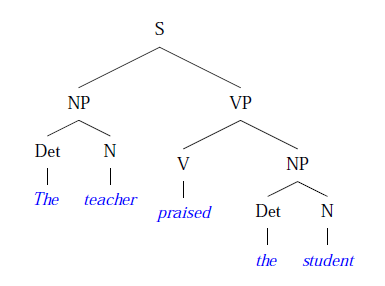
Alternatively, labelled bracketting may be used.

Using phrases, rather than specifying grammar rules in terms of all possible POS tag combinations, allows us to better generalise the possible patterns underlying the sentences.

Phrases bearing the same category exhibit similar distributional behaviour, i.e., may appear in roughly the same contexts. Distributional similarity is tested by substitution (i.e., substituting one for another in a range of contexts preserves grammaticality).

When talking about PSG trees, there is some terminology that can be used. A node X dominates node Y in a tree iff there is a path down from X to Y. Node X immediately dominates node Y in a tree iff X dominates Y and there are no intervening nodes on the path between. A local tree is a tree or subtree licensed by a single phrase structure rule.

Various phrasal category names make reference to a lexical category (e.g., noun phrase). This element is considered to be the head of the phrase. The head principally determines the character of the phrase, and thereby its distribution - the phrase and the head have similar semantic 'feels'.

A head may require other phrases to appear alongside it, called the complements. The complements a head requires is related to its meaning. Complements are often obligatory, but some are optional.

Heads may be further classified in terms of the patterns of complements which they allow - this classification is known as subcategorisation, and a head is said to subcategorise for its complements.

Adjuncts are phrases that supply additional information about events or entities, and their presence is always optional, and often multiple adjuncts are allowed. An adjunct is said to modify the phrase with which it is associated. Self-recursive grammar rules allow for optionality and multiple occurences.

Noun Phrases

Verb Phrases

Basic Sentence Structure

Prepositional Phrases

Clausal Complements and Adjuncts

Adjective Phrases

Adverbial Phrases

The assumption that we can capture a word's syntactic behaviour by assigning it lexical categories which are simple atomic symbols causes issues. There exists phonomena that shows the simple PSG approach is inadequate for handling real language.

If we recall the criterion of distributional similarity for determing the category a word should be placed in, which can be tested by substitution, then we find contexts where words that have been previously considered distributionally similar can no longer be substituted and grammaticallity remains.

We can separate these words out into separate classes, but then generalities about contexts in which they behave similarly are lost, resulting in many extra grammar rules. However, if they are retained in a common category, then the grammar will overgenerate.

A better solution is to provide a means of further subclassifying units into subcategories (e.g., with singular and plural NPs being subcategories of the NP category). This can be done by replacing the atomic category symbols of a simple PSG with feature-based representations called feature structures.

A feature structure is a set of feature-value pairs which together describe a category. Some examples of possible features are case or number.

PATR Notation

Feature Matrices

In English, virtually any two types of phrase can be co-ordinated using a co-ordinating conjunction.

By using feature representations, co-ordination can be captured by a single rule to enforce categories on both sides of the conjunction match, and the overall category of the conjunction is that of those categories. An additional feature equation is used to require that the co-ordinated items have the same subcategorisation requirements.

Tense and aspect in English are largely indicated through the use of auxiliaries. We can use a feature 'vform' to identify the form of the verb with values such as 'finite', 'present_participle', etc. Specific auxiliaries both require that the verb group following has a certain vform, and determine the vform of the verb group being produced. Lexical entries for each auxiliary might record both the following and resulting verb forms using the two features vform and rvform.

Simple verb phrase rules then pass up their vform value, and a grammar rule is also required for auxiliaries that appropriately checks the vform values and passes the rvform values.

A simple PSG can easily express dependencies between sibings, but not between non-siblings. If we consider the rules A → (B) C and C → (D) E, where brackets indicate optionality, then these rules encode the local dependency if B is present, then so is C', but they cannot encode non-local dependencies, such as 'if B is present, then D is present', or 'if B is present, then D is absent'.

Subject-verb agreement is one example of non-local dependency. Another, more striking, example is provided by unbounded (or filler-gap) dependency constructions.

An example of this is "Who does John admire?", vs. the sentence "Does John admire Mary?". We can therefore determine that the object of 'admire' can be absent, and the extra word 'who' may appear before the clause. However, consider 'Who does John admire Mary?'. We therefore determine that who is present iff the object NP is absent. A simple PSG can not capture this non-local dependency.

In such constructions, the site of the missing phrase (the object NP) is called the gap. The semantically corresponding, but displaced, phrase is called the filler. Hence, such constructions are often called filler-gap constructions.

The dependency between the filler and the gap may extend across any number of sentence boundaries, hence such constructions are alternatievly known as unbounded dependency constructions, or UDCs. Some key types of UDCs are wh-questions, relativisation, topicalisation and extraposition.

wh-questions invite more specific answers than just yes or no. They begin with a wh-phrase (i.e., one that includes a wh-word, such as who, what which, but can also include other words, such as "To whom" or "Which writer"). In main clause wh-questions, subject-auxiliary inversion is required, except where the wh-phrase corresponds to the subject. But, such inversion is not required in embedded questions.

Relative clauses are embedded clauses that serve as noun modifiers (i.e., akin to adjectives). They are introduced either by the relative pronoun that (e.g., this is the book that I bought), or a wh-item (e.g., this is the book which I bought), or sometimes there is no initial filler item (e.g., this is the book I bought).

Subject and complement relatives are distinguished depending on whether the gap site is the subject or some verb complement.

wh-questions and wh-relatives together are referred to as wh-constructions. They together suggest a need for a uniform treatment of filler-gap dependencies.

In topicalised sentences, a non-wh NP appears in sentence initial position (e.g, "Beans, I like!"). Topicalised sentences can only be used in certain contexts, and tend to have unusual intonation (i.e., the part of utterance stressed).

Extraposition is a general term used by linguists to denote phrases moved away from their normal context (topicalisation can be seen as one type of extraposition). Such phrases can include prepositional phrases ("To the soup he had added basil"), or NP complements/modifiers ("A paper was written examining Chomsky's position").

UDCs have three crucial components that an account must address: the gap (or extraction) site, the filler (or landing) site, and the transmission of the dependency between the filler and the gap.

One proposal for handling UDCs within a PSG employs so-called slash categories. A category X/Y represents a phrase of category X which is 'missing' a phrase of category Y.

The gap site allows for the empty string ε to have a category such as NP/NP by a special lexial entry (or PSG rule). The filler site is handled directly with a PS rule allowing a phrase Y to appear beside another of category X/Y.

The dependency must also be transmitted. This is done by allowing special 'gap transmitting' variants of other PSG rules in the grammar (e.g., where the grammar has a rule X → Y, allow extra rules of the form X/NP → Y/NP). Such extra rules can be created by a meta-rule (a higher level rule which describes the grammar rules).

A feature 'slash' can be used for transmission of the gap information. The value here is the category of the missing phrase, or 0 if there is none. Relativisation rules allows for the filler to appear, and other rules must allow for the transmission of the slash value.

Feature structures are representationally powerful, but of little use if we cannot perform operatons on them. In particular, we want to compare information in feature structures, merge information in feature structures if they are compatible, and reject mergers of feature structures if they are incompatible.

An important relation between feature structures is subsumption. A feature structure F₁ subsumes another feature structure F₂ iff all the information contained in F₁ is also contained in F₂.

Two features may be such that neither subsumes the other. The subsumption relationship between feature structures is somewhat similar to the subset relation between sets.

Subsumption is an important concept for defining unification - the operation of combining feature structures such that the new feature structure contains all the information in the original two and nothing more.

Unification is a partial operation - i.e., it is not defined for some inputs. For example, if there is conflicting information between two features (for example, each feature matrix contains 'cat' and the contents are set to be different categories), then there can be no feature structure that contains the information from both, and unification fails.

Formally, the unification of two feature structures F and G, if it exists, is the smallest feature structure that is subsumed by both F and G. i.e., F unified with G, if it exists, is the feature structure with the properties of: F unified with G is subsumed by G; F unified with G is subsumed by F; and if H is a feature structure such that F subsumes H and G subsumes H, then the unification of F and G subsumes H.

Unification-based Chart Parsing

Computational syntax deals with issues of how best to represent syntactic information in a computer, and how best to apply it in the process of analysing natural language sentences (parsing), or producing them (generation).

Syntactic analysis can be used directly in applications such as grammar checking in word processing software. More usually, a syntactic analysis, such as a parse tree, is an intermedia stage of representation for semantic analysis.

Syntactic analysis can play a role in applications such as machine translation, question answering, information extraction and dialogue processing.

See TOC for
a formal CFG definition.

A common grammar formalism used is that of a context-free grammar. A language is then defined via the concept of derivation: one string is derived from another if the latter can be rewritten via a series of production rule rewrites into the former.

Parsing suffers from the issue of ambiguity, as already seen in relation to POS tagging. Structural ambiguity arising from multiple possible grammatical analyses is also pervasive in natural languages.

One common form of structural ambiguity is attachment ambiguity, which occurs when a constituent can be attached to the parse tree in more than one place. Another common form is co-ordination ambiguity, which occurs when different sorts of phrases can be conjoined by a conjunction.

The problem of structural ambiguity is common and serious. In the case of multiple attachments, the number of possible parses grows exponentially in the number of attached phrases. This is a problem that affects all parsers, due to the nature of the grammar.

To choose the correct parse (syntactic disambiguration) is a process that may require semantic/world knowledge, statistical information (probability of that parse being chosen) or discourse information (coreferences mentioned earlier in the text). Without such knowledge, all a parser can do is return all parses, or accept incompleteness (giving up after depth or time bounds are met).

A grammar tells us what the allowable phrase structures are, but not how to find them. To build a parser (or recogniser), we need a control mechanism or search strategy that tells us how to go about finding the structures which a grammar permits (i.e., a search strategy which tells us which rules to apply to which substrings of the sentence and in which order). Thus, to parse, we need both knowledge of grammatical structure, and a control stategy.

Three key dimensions for classifying parser strategies are left-to-right vs. right-to-left, top-down vs. bottom-up, and depth-first vs. breadth-first.

In a left-to-right parser, parsing starts at the left, and proceeds rightwards, and vice versa for a right-to-left parser. Most language which are written left-to-right also proceed left-to-right, but there is nothing which requires this.

Given a grammar and an input, a parser might proceed in either of the following ways to find a parse: top-down, or bottom-up. In a top-down strategy, we start with the grammar's top category and expand it, followed with daughters, etc, until the top category has been expanded to give the input. A bottom-up approach starts with the input, replacing lexical items with lexical categories, and then looking for subsequences of categories matching the righthand side of the rules, replacing them with their lefthand sides, and so on, working towards the top category.

Top-down parsing has the disadvantage of hypothesising phrases that are impossible, because requisite lexical items are not present in the input, and may fail to terminate if the grammar includes left-recursive rules. However, it will never attempt to construct phrases in contexts in which they can not occur.

Bottom-up parsing may try to construct constituents that can not occur in the given context, however never attempts to build constituents that can not be anchored in the actual input.

In depth-first search, each hypothesis is explored as far as it can be explored before exploring any others. The alternative method, breadth-first search, explores each hypothesis once, and then continues onto sibling hypotheses.

Recursive Descent Parser

Chart Parsing

Human langauge ability is productive. We can produce/understand indefinitely many different sentences, but cannot have memorised meaning of all understandable sentences. This suggests that we have some means to compute the meaning of each sentence. An influential view of how this is done is attributed to 19th century German philosopher/mathematician Gottlob Frege. This view is summed up as the principle of compositionality, or Ferge's principle.

The principle of compositionality states that the meaning of the whole is a function of the meaning of its parts, and their mode of composition. i.e., so that the meaning of a sentence of determined by the words present, and how they have been put together to form the sentence.

It is possible that what is the semantically relevant mode of composition of a sentence might be something other than its syntactic structure, but one view is that the semantically relevant structure is precisely its syntactic structure. This leads to an interpretation of the principle of compositionality whereby the meaning of a complex expression depends on those of its subconstituents and the syntactic rules used.

This view is most strongly stated as the rule-to-rule hypothesis: corresponding to each syntactic rule which states how a phrase can be constituted, there is a semantic rule which states how the meaning of such a phrase is composed out of the meanings of its syntactic components.

Construed in this way, compositionality places severe constraints on the admissable systems of syntax and semantics.

In the study of formal semantics, the concern is to derive a representation of sentences in some logical formalism. This logical representation should capture the truth conditions of the original sentence.

The study of formal semantics is most closely associated with Richard Montague, hence, a formal semantic approach is sometimes called Montague semantics, or Montagovian semantics. This 1974 book Formal Philosophy set out a programme whose goal was the translation of all of natural language into a suitably powerful logical language.

Montague thought natural language semantics could be handled using essentially the same ideas and techniques as was used in handling the semantics of the formal languages of logic, and years of NLP research have underlined the importance of inference to language understanding. Logical formalisms have well-defined computational inference procedures.

Montague employed an extremely powerful logic - a higher order intensional logic based on the typed lambda calculus. In this module, a much simpler logic is used that conveys the essence of the approach.

The approach we take is representational (derivations yield a "meaning representation", or logical form, for the sentences), truth-conditional (semantic representations capture meaning by having well-defined truth-conditions) and compositional (meaning representations are contructed from lexical meanings via syntactic derivation in a rule-to-rule fashion).

The semantic representation for complete sentences will initially be first-order predicate logic, but the rule-to-rule approach requires us to be able to associate meaning representations with all subconstituents. Therefore, we need some additional apparatus to be able to build meaning representations for smaller units than entire sentences.

Firstly, we use a convention of using primed variants of words to represent its meaning (e.g., run′ for runs). So, the sentence John runs may have the semantics of run′(john′). Presumably, the verb contributes the predicate run′ and the NP contributes the atomic constant john′ to this meaning. The meaning of the is also presumably just run′.

If we consider the phrase 'John likes Bill', this may have the semantics like′(john′, bill′), with the verb contributing the predicate and the NPs the constants. But what is the meaning of the VP "likes Bill"?. It would be something like like′(_, bill′), but this is not a well-formed formula, and it is not obvious how it is subsequently to be completed.

These incomplete meanings can be usefully treated as functions. A method is therefore needed to construct functional expressions on the fly. This is called lambda calculus.

The expression "x + 2" could stand for either a function, mapping from any particular value for x to give x + 2, or the value of that function at some particular x.

To unequivocally denote the function, we write &lamda;x.x+2. The λ operator is said to bind its variable. This process is called λ-abstraction.

An λ-expression can be used anywhere an atomic functor might, e.g., (&lamda;x.x+2)(2) = 4. Additionally, multiple abstractions are allowed for multiple variables.

We can state schematic equivalence for λ-calculus. (&lamda;v.φ)(t) = φ[t/v], where φ[t/v] is the result of substituting t for v in φ. This equivalence can be used for simplifying expressions, e.g., (&lamda;x.x+2)(3) to 3 + 2. This simplifying step is known as beta-reduction (or beta-conversion or lambda-conversion).

With each rule in the grammar and word in the lexicon, a semantic rule is associated. e.g., for S → NP VP, the semantic rule VP′(NP′) is associated. This shows how to build the meaning of the parent constituent from the meanings of the child constituents.

Co-ordination and negation rules can be handled in the same way. e.g., for conjunctions, the syntactic rule Conj′(S₁′)(S₂′) is used, and the different conjunctions should have the semantics of, e.g., λsλt.(s ∧ t) for and, and λsλt.(s ∨ t) for or.

If we consider the sentence 'Every student walks', then the natural representation in FOL is ∀x(student′(x) → walk′(x)).

The quantifier ∀ has a wide scope (the scope extends to the semantics of the VP), and such a semantics cannot be produced in an approach where the VP meaning is a function over the subject NP meaning. e.g,. the VP semantics λy.walk′(y) would always produce a result of the form walk′(T).

One solution is to change the syntax and semantic rules so that NP meaning is a function over VP meaning, i.e., S → NP VP : NP′(VP′). Suitable semantics for the subject NP is then λp.∀x.(student′(x) → x). The resulting NP′(VP′) simplifies appropriately.

Previously, proper nouns have been treated simply as atomic terms, however have switched to having NP semantics be a function over VP semantics, treatment must be modified. The same final semantic representations as before can be achieved by giving proper nouns a different logical form, e.g., for 'John', λq.q(john′).

For existentially quantified NPs, essentially the same approach can be taken. e.g., for existentially quantified NP "a student", using the same reasoning as above, the semantics would be: λp.&exists;x.(student&prime(x) ∧ p(x)). Likewise, we can define the semantics for the determiner 'a' as: λq.λp.&exists;x.(q(x) ∧ p(x)).

"No" as in "no cat swims" can be translated into FOL using negation and either universal or existential quantification: λq.λp.¬&exists;x.(q(x) ∧ p(x)) or λq.λp.∀x.¬(q(x) ∧ p(x)).

The handling of VPs with transitive verbs must also change. A simple inversion as before is not possible, as VPs are functions requiring one argument, and TVs require two. Applying an NP meaning to a TV meaning produces non-sensical results, where abstractions for variables get trapped inside terms and cannot be linked to the subject NP by the S rule.

TV′ can be modified into a suitable argument for NP′ by building the partial function λu.TV′(u). This is now a partial function requiring one argument - its object. The complete modified TV rule is hence: VP → TV NP : λw.NP′(λu.TV′(u)(w)).

Using the semantic rules developed so far, we can handle multiple quantifiers. For example, the sentence "Every student likes a book" allows a reading that the book liked by each student may differ (as long as each likes at least one). However, the alternate reading of a single book being liked by all students can not be derived.

Alternative readings of a sentence may differ considerably in plausibility, but without using contextual information or world knowledge, it is in general impossible to tell which reading is intended. One view is that the formal account should generate all possible quantifier scopings, assuming some subsequent process evaluates alternatives to determine the most plausible.

So far, only a small number of determiners/quantifiers - those that naturally translate to FOL quantifiers - have been discussed, but natural language contains a host of additional quantifiers, called generalised quantifiers. These go beyond the classical existential and universal quantifiers and add quantification such as one, two, few, many, no more than five, etc. Many of these cannot be translated into standard FOL.

Classical quantifiers involve quantification over the whole domain. However, if we consider the natural language quantifier "most", then we could define a new quantifier M such that Mx.φ is true iff φ is true when x = d for more than half of the individuals d in the domain.

However, even with this quantifer, defining "Most dogs bark" is problematic. Mx.(dog′(x ∧ bark′(x))) paraphrases as "most x are such that x is a dog and x barks". This could be false even when all dogs bark, if more than half of the domain are non-dogs.

Similarly, Mx.(dog′(x) → bark′(x)) paraphrases as most x are such that if x is a dog, then x barks. This could be true even if no dogs bark, e.g., if more than half the domain are non-dogs.

Other connectives fare no better in combining dog′(x) and bark′(x) as terms to be quantified with M. Research into the interpretation of NL quantifiers is general is addressed with generalised quantifier theory.

A key insight is that the meaning of NL quantifiers involves reasoning about sets of individuals, where these sets are picked out by NL expressions. That NL quantifiers are concerned with a restricted set of indivudals is in contrast with FOL quantifiers, which involve quantification over all individuals in the domain.

In 'most dogs bark', the quantifier 'most' relates two predicates - the meanings of the expressions dogs and barks. Set comprehensions can be used to determine corresponding sets of individuals. e.g., for dogs, this is {x | dog′(x)}. This set is referred to as the extension of the predicate.

In our example of "most dogs bark", we can compare the set of dogs with the set of things that bark, and require that some suitable proportion of the former are also members of the latter. This can be expressed as a requirement on sets such as: |{x | dog′(x)} ∩ {x | bark′(x)}| / |{x | dog′(x)}| > 0.5

Standard generalised quantifer notation combines components without a logical connective. e.g., for "most dogs bark", we can represent this with the formula: most(x, dog′(x), bark′(x)). In this example, the second argument is called the restriction (or range) and the third argument is called the body (or scope). Quantified formulae take the general form: quantifier(variable, restriction, body). This approach is called the 'three-branch' quantifier notation.

The condition capturing the meaning of an NL quantifier typically refers to the intersection of the restriction and body extension sets, i.e., for quant(x, R(x), B(x)), the condition will mention the set {x | R(x)} ∩ {x | B(x)}, or equivalently {x | R(x) ∧ B(x)}. The condition either restricts the set directly, or compares it to the set {x | R(x)}.

This set comparison approach works for the cases handled by standard quantifiers, so existential and universal quantification can be handled with the new notation, e.g., every: {x | R′(x) ∧ B′(x)} = {x | R′(x)}; some: {x | R′(x) ∧ B′(x)} ≠ ∅; no: {x | R′(x) ∧ B′(x)} = ∅

NL quantifiers can relate predicates taht are complex (that is, more than just single atomic predicates) and who do not appear in subjects. This can be captured using this notation.

Relative clauses serve as noun modifiers, giving rise to a meaning that is a conjunction of the noun's meaning with some other property (note that the term property is used to refer to single argument functions from individuals to truth values).

For a subject relative, the additional property is simply the meaning of the VP making up the relative clause. These basic subject relatives can be handled straightforwardly by the rule: RelC → Rel-Pro VP : VP′, so the relative clause meaning is identical to that of the embedded VP. A further rule is needed to allow the relative clause to modify N: N → N RelC : λx.(N′(x) ∧ RelC′(x)). This creates a conjoined property from the two component meanings.

For complement relatives, additional properties to conjoin with the noun meaning is produced by abstracting over a variable appearing in the semantic position corresponding to the gap site.

To interpret such a structure, you can assign a variable for the semantics of the gap site, and then abstract over that variable when the filler site is reached.

However, the identity of the variable to bind also needs to be remembered. This can be stored with the slash information, as the value of some feature. For convenience, the notation (e.g.,) NP/NP_u is used for NP with the slash value NP and u as the associated variable.

This gap can be generated by a rule such as NP/NP_u → ε : λs.s(u), and then filled at the filler site with a rule such as RelC → Rel-Pro S/NP_u : λu.[S/NP]′. For transmission of slash dependencies, the rules need not change.

The semantics of a wh-question might be a property which is true of those things which are correct answers to the question. e.g., the meaning of "Who likes Bill?" is the property λx.like′(bill′, x), which corresponds to the semantics of the VP "likes Bill".

This suggests the following rules for the subject and complement wh-questions: Q → Wh-Pro VP : VP′ and Q → Wh-Pro Sinv/NP_u : λu.[Sinv/NP]′. We can assume there are also rules for subject-aux inverted sentences (Sinv), with and without gap transmission.

For yes/no questions formed from sentences involving subject-aux inversion, the meaning returned might be the same as for the corresponding declarative sentence. If we wanted an approach where the semantics of questions was a function returning true for values that are correct answers to the question, a term could be built, such as: λx.((x = 'yes' ∧ Sinv′) ∨ (x = 'no' ∧ ¬Sinv′)). Alternatively, we might just mark simple semantics in some way to distinguish it from declarative semantics.

For both wh- and yes/no questions, meaning representations could be used in formulating queries against a logic database in a question answering system.

Formal semantics deals with meaning representations for full sentences, showing how the meanings of syntactic wholes could be built out of parts (phrases, words, etc). In this approach, meanings of individual words are largely ignored, though Montague believed some of the meaning of words is captured through meaning postulates - axioms relating one logical predicate to the other (e.g., ∀x author′(x) ⇒ &exists;y book(y) ∧ write(x, y)).

Formal semantics leads to a view of the lexicon as a list of words without any systematic structure, when in fact there is a rich structure of semantic relations between words, and internally between different meanings of individual words. This field of stufy is called lexical semantics.

It is useful here to work in terms of lexemes, rather than words. Lexemes are individual entries in the lexicon, and can be thought of as a pairing between an orthopgrahic and phonological form, and a sense of meaning component.

It is useful to distinguish various semantic relations that can hold amongst lexemes.

Homonymy

Polysemy

Syonymy

Hyponymy

WordNet is a large, freely available lexical database of English words containing nouns, verbs, adjectives and adverbs grouped into sets of cognitive synonyms, called synsets, each expressing a distinct concept.

Two entries are considered synonyms if they can be successfully substituted in some context, and synsets are interlinked by means of lexical semantic relations.

Word Sense Disambiguation

Montague concentrated on the treatment of single sentences. His treatment of indefinite quantifiers (a, an, etc) used the existential quantifier. However, variables are bound by the quantifier and are not available outside the logical expression. Therefore, any x occuring in another expression is not related to the same thing the x in a single sentence refers to.

Most NL texts, however, have multiple sentences, and multiply refer to the same entity. Existentially quantified variables are not well-suited for this task. This suggests we need some representation of discourse referents - a means of naming and subsequently referring to these entitites that persist between sentences.

The study of reference in philosophy and linguistics addresses how words and phrases in sentences connect to objects in the world. In NLP, study of reference addresses how phrases (commonly NPs) identify new or existing objects in our model of the text's meaning.

NP references can be divided into two forms: anaphoric, where the NP refers to an object previously mentioned in the text; and non-anaphoric, where the NP identifies an object not previously mentioned. An anaphoric NP is called an anaphor, and the other NP is called the antecedent. Two such NPs are said to corefer.

Not all coreferences involce NPs, however. Pronouns (e.g., it) can do as well. A simple view that NPs either refer to previously mentioned objects or introduce new ones. In English, determiners may be used to signal this distinction. Indefinite references introduce new objects into the context (e.g., determiners such as 'a' or 'some'), and definite references refer to objects previously introduced (e.g., determiners such as 'the' or 'these').

However, this simple view is too simple. For example, sets of things can be introduced, and then single members of it referred to, or whole objects introduced and parts of it referred to. Additionally, there are also cases where determiners such as 'the' are not reliable indicators of previously introduced objects.

Aside from determiners, other syntactic constraints can help to identify coreferents. Antecedents and anaphors must agree in number, person and gender, and if the anaphoric pronoun is the object of a clause whose subject is the antecedent, then the pronoun must be reflexive (e.g., "Narcissus saw him in the pool" vs. "Narcissus saw himself in the pool").

Anothey key distinction is between intrasentential anaphora, those where the anaphor and antecedent are in the same sentence, and intersentential anaphora, where the antecedent and anaphor are in different sentences.

Pronominal anaphora is one type of anaphoric reference. This involves the use of a pronoun, such as he, she or it, or a possessive pronoun such as hers or a reflexive pronoun such as himself. The pronoun usually follows the NP with which it corefers, but not always. When it doesn't, this sort of forward reference is called cataphoric references.

One-anaphora uses words like one or some to introduce new objects in the same class as those previously introduced (e.g., "John had a pint of Guiness. I had one too.").

Set/set member anaphora involves phrases which introduce a set of objects, following by another phrase which refers to an individual in the set. Typically, the expression introducing the set appears first, and the expression referring to the individual in it later, but this is not always the case.

Part/whole anaphora involves a phrase which refers to part of an object introduced by another phrase. Typically, the expression introducing the whole appears first, and the expression referring to a part of it appears later.

VP and Sentence anaphora involve references to events or activities identified by a whole sentence or a VP.

Apposition is when two NPs placed adjacently are frequently used to introduce two descriptions of the same individuals.

Related object anaphoric reference occurs when frequently associated objects are referred to before they have been introduced.

These categorisations are not exhaustive, and it may be possible to categorise the same phenomena in different ways.

Various flexible semantic representation languages have been proposed for NLP purposes. Allen presented a quasi-logical form language which permits ambiguity to be perserved for multiple word senses, and leaves quantifier scopes unresolved. Alshawi also presented a quasi-logical form langauge, called QLF, in which quantifier scopes and pronoun referents are unresolved.

Here, we consider a simplified quasi-logical form language called S-QLF, in which every NP names an individual object (which may be a set), every VP names an individual event, quantifiers are left uninterpreted and scopes are not resolved, and word sense ambiguities are not resolved (morphological roots of content words are used as predicates in meaning representations), and predicates are used which are the morphological roots of key words.

For example, "The knight loved the lady in the tower" is represented in S-QLF as knight(r1) & det(r1, the) & love(e1) & time(e1, past) & lsubj(e1, r1) & lady(r2) & det(r2, the) & lobj(e1, r2) & in(r2, r3) & tower(r3) & det(r3, the). Here, lsubj stands for logical subject - the object that carries out an action (comparable to a relation sometimes called an agent) - and lobj stands for logical object - the object that is affected by an action, or to which the action is directed. These notions are separate from the usual notions of syntactic subject and object, however, S-QLF representations of the passive sentence is identical to that for the active.

The use of event identifiers, such as love(e1) allows for easy reference to the event. For example, to modify an event, all that needs to be done is a single element to be added, e.g., manner(e1, obsessive) to indicate that the knight obsessively loved the lady in the tower. This is 'Davidsonian' treatment of verb semantics, where event identifiers name the event introduced by a verb instance, and all associated information are predicated of that identifier.

In S-QLF, this is the typical treatment of prepositional phrases - binary predicates where the predicate name is the preposition, the first argument is the identifier of the event or object qualified by the PP, and the second argument is the identifier of the complement of the preposition.

We can see, therefore, that S-QLF uses discourse referents for entities referred to, or quantified over, by NPs, and named entities are labelled, so they can be referred to over and over.

S-QLF therefore allows us to refer to the same individual across multiple sentences using discourse referents. This is important for representing dialogue - a task scoped quantifiers are not well suited to. Additionally, Davidsonian event semantics provides a common basis for representing the meaning of a verb with multiple subcategorisation frames. This helps identifying common meaning between different forms, and is also useful for robust parsing (i.e., if only some of the verb's complements are found).

The Montague-style semantic approach of using unambiguous logical forms is problematic as language is highly ambiguous, resolutions may not be possible on the basis of context, and a large number of alternative meanings may need to be computed. S-QLF does not resolve these various forms of ambiguity (disambiguating word senses or attempting to encode quantifier scopes).

The problem of identifying which expressions in a discourse corefer is called coreference resolution. Various types of information and knowledge can be used in this task.

In some cases, a type of anaphora is strongly associated with a particular syntactic structure. Then, successful parsing may be sufficient to resolve a coreference relation. For example, a reflexive pronoun in the object position of a transitive verb always corefers with its subject, but a non-reflexive pronoun in the same position does not corefer with the subject. In the latter case, this syntactic constraint only serves to rule out one otherwise possible coreference, and is not in itself sufficient to resolve the coreference of the pronoun.

Another case where coreference resolution is clear is in apposition structures - two adjacent NPs always corefer. However, this task is still non-trivial. The structure must be found and determined whether or not it is it eh right one, even when the sentence is structurally ambiguous.

For syntactically resolvable coreference relations, the key knowledge source enabling resolution is a grammar. This may be a PSG with or without feature representations, or some other form of grammar.

Syntactic knowledge may be useful, and sometimes even sufficient, for resolving coreference - however, in general, syntactic knowledge is not sufficient to permit coreferences to be correctly resolved, we still need conceptual or world knowledge. To bring such knowledge to bear on the problem of resolving coreference, we need a means of representing such conceptual and world knowledge, and an algorithm for using it to build a coherent meaning representation for a discourse from the meaning representations of individual sentences.

There is also the problem of how to acquire this knowledge in the first place, but this is not addressed here.

In general, coreference resolution requires a search process(i.e., consider alternative possible antecedents, and select the best on the basis of a number of possible criteria). This coreference process applies to discourse referents (DRs) of anaphoric expressions.

For each such referent, we can computer candidadates(r) - the set of all candidate antecedents for r. This might be all other (i.e., ≠r) DRs in the same sentence, and all preceeding sentences of discourse, or it may be more limited (e.g., only DRs of the current or preceeding sentences within the same paragraph). The algorithm then simply computes a resolve_score between r and each candidate antecedent, and selects the highest scoring candidate. The problem then reduces to computing a resolve score between two DRs, which might be 0 if definitely distinct, 1 if definitely identical, or in between those for all other cases.

The factors that may contribute to preferring one possible antecedent over another are what needs to be considered in order to compute the resolve_score values.

Type Compatibility

Attribute Compatibility

Recency