Theory of Computation

TOC is an extension of MCS , and as such extends on the topics originally covered in MCS, such as:

Inductive proofs and definitions (also covered in ICM)
Finite automata
Kleene's Theorem
Non-deterministic finite automata
Grammars
Regular grammars
Context-free grammars
Pushdown automata
Chomsky hierarchy

Level	Grammars/Languages	Grammar Productions	Machines
0	Unrestricted/recursively enumerable	α → β [α ∈ (V ∪ Σ)⁺, β ∈ (V ∪ Σ)*]	Turing Machine
1	Context-sensitive	α → β [α, β ∈ (V ∪ Σ)⁺, \|α\| ≤ \|β\|]	Linear-bounded automaton
2	Context-free	A → β [A ∈ V, β ∈ (V ∪ Σ)*]	Pushdown automaton
3	Regular	A → a, A → aB, A → Λ [A, B ∈ V, a ∈ Σ]	Finite automaton

We could also consider a level 2.5, which is a deterministic context free grammars.

Context-Sensitive Languages

A grammar is context sensitive if α → β satisfies |α| ≤ |β|, with the possible exception of S → Λ. If S → Λ is present, then S must not occur in any right-hand side. The length restrictions here mean that you can generate all strings in a language up to a certain length (derivation trees).

Context-sensitive grammars generate context-sensitive languages, and every context free language is context sensitive.

Linear Bounded Automata

A linear bounded automata (LBA) is defined like a nondeterministic Turing machine (see next section), M, except that the initial config for input w has the form (q₀, <w>) and the tape head can only move between < and >.

An equivalent definition allows inital configurations of the form (q₀, <wΔⁿ>), where n = c_M|w|, for some constant c_M ≥ 0. This allows to have multi-track machines, where c_M represents the number of tracks.

Theorem: A language L is context sensitive if and only if L is accepted by some LBA.

Open research problem: Are deterministic linear bound automata as powerful as non-deterministic LBAs?

Turing Machines

Turing machines were introduced by Alan Turing in "On Computable Numbers with an Application to the Entscheidungsproblem" (The Entscheidungsproblem is whether or not a procedure of algorithm exists for a general problem).

A Turing Machine is an automata with consits of a 5-tuple (Q, Σ, Γ, q₀, δ)

Q is a finite set of states including h_a and h_r (the halting accept and reject states)
Σ - the alphabet of input symbols
Γ - the alphabet of tape symbols, including the blank symbol Δ, such that Σ ⊆ Γ - {Δ}
q₀ - the initial state, such that q₀ ∈ Q
δ - the transition function such that δ : (Q - {h_a, h_r}) × Γ → Q × Γ × {L, R, S}

Intuitively, a Turing machine has a potentially infinite set of squares and a head moving on a type when reading character a whilst in state q, δ(q, a) = (r, b, D), which denotes a new state r, a is overwritten with b and the head either moves to the left (D = L), right (D = R), or remains stationary (D = S).

Configurations and Transitions

A configuration is a pair (q, uav) where q ∈ Q, a ∈ Γ and u, v ∈ Γ*. This configuration is considered to be the same as (q, uavΔ) - the rightmost blanks can be ignored.

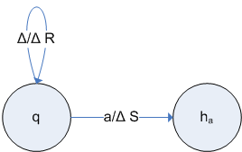
A transition (q, uav) ├ (r, xby) describes a single move of a Turing machine, and we can write (q, uav) ├* (r, xby) for a sequence of transitions. This can be represented diagramatically as:

Convention also dictates that if there is no transition for what you want to do, a transition to h_r is implied.

There are also special case transitions we can use:

The initial configuration for input w ∈ Σ* is (q₀, Δw)
Configuration (q, xay) is a halting configuration if q = h_a or q = h_r, an accepting configuration if q = h_a and a rejecting configuration if q = h_r.
Tape extension at the right end: (q, va) ├ (r, vbΔ) if δ(q, a) = (r, b, R) for some r ∈ Q and b ∈ Γ.
A crash occurs at the left end of the tape: (q, av) ├ (h_r, bv) if δ(q, a) = (r, b, L) for some r ∈ Q and b ∈ Γ.

The language accepted by the Turing machine M is L(M) = {w ∈ Σ* | (q₀, Δw) ├* (h_a, xay) for some x, y ∈ Γ* and a ∈ Γ}

Non-deterministic Turing Machines

A non-deterministic Turing machine (NTM) varies from the Turing machine in the transition function. δ: (Q - {h_a, h_r}) × Γ → 2^{Q × Γ × {L, R, S}}

Theorem: For every NTM N, there exists a TM M such that L(M) = L(N)

Multi-tape Turing Machines

Intuitively, this is a machine with n tapes on which the machine works simultaneously. This is defined like the Turing machine, which has a revised definition of the transition function. δ: (Q - {h_a, h_r}) × Γⁿ × {L, R, S}ⁿ, where n ≥ 2.

Configurations on a multi-tape machine have the form (q, u₁a₁v₁, u₂a₂v₂, ..., u_na_nv_n), and the intial configuration for an input w is (q₀, Δw, Δ, ..., Δ), by convention.

Theorem: For every multi-tape machine N, there exists a TM M such that L(N) = L(M).

Recursively Enumerable

A language L is recursively enumerable if there exists a Turing machine that accepts L.

Theorem: A language L is recursively enumerable if and only if L is generated by some (unrestricted) grammar.

Enumerating Languages

A multitape TM enumerates L if:

the computation begins with all tapes blank
the tape head on tape 1 never moves left
at each point in the computation, the contents of tape 1 has the form Δ#w₁#w₂#...#w_nv, where n ≥ 0, w₁ ∈ L, # ∈ (Γ - Σ) and v ∈ Σ*
Every w ∈ L will eventually appear as one of the strings w on tape 1.

Theorem: A language L is recursively enumerable if and only if L is enumerated by some multitape Turing machine.

Computability

Decidability

A language L is decidable (or recursive) if it is accepted by some Turing machine M, that on every inputs eventually reaches a halting state (h_a or h_r), i.e., it does not get stuck and loop. We say that M decides L.

To decide whether w ∈ Σ* is in L, we run M on w until M reaches a halting configuration, then w ∈ L if and only if M is in state h_a.

Theorem:

Every context sensitive language is decidable - however as the converse is not true, we can consider decidable languages as level 0.5 on the Chomsky hierarchy.
If a language L is decidable, then the complement L = Σ* - L is also decidable
If both L and L are recursively enumerable, then L is decidable

Proof of Theorem 2

Let M be a Turing machine that accepts L and reaches a halting config on every input (is decidable). Modify M to machine M as follows.

Swap h_a and h_r by defining h_a = h_r and h_r = h_a.
Put a new symbol at the start of the string (to detect the crash condition)
1. Shift existing string one position to the right
2. Put a special symbol (e.g., #) at the first square
3. Move tape head to the second square (the old first square)
4. Continue as for a normal TM
5. δ is extended as δ(q, #) = (h_a, #, S) ∀ q ∈ Q.

Therefore, L(M) = L(M), and L is decidable, as neither of the modifications described above can introduce looping.

Proof of Theorem 3

Intuitively, L(M) = L and L(M) = L. For a string w, w ∈ L ∨ w ∈ L - so at least one of those machines will accept the string. If the two machines are run in parallel and terminate as soon as one reaches an accept state, then it is impossible to get into a loop. This can be accomplished on a two-tape machine. The string is copied to tape 2 in the first instance, and then M is run on tape 1 and M is run on tape 2.

We can express this formally as: Let M = (Q, Σ, Γ, q₀, δ) and M = (Q, Σ, Γ, q₀, δ) be Turing machines that accept L and L respectively. Without a loss of generality, we can assume that M and M cannot crash at the left end of the tape.

We can construct a two-tape Turing machine M′ that decides L by copying its input to tape 2 and simulating M and M in parallel.

Let Q′ ⊇ Q × Q (we need additional states for initial copying, which are Q′ - (Q × Q)).
Let δ′((q, q), (x, x)) = ((r, r), (y, y), (D, D)), where δ(q, x) = (r, y, D) and δ(q, x) = (r, y, D). Also, we need to define:
1. δ′((h_a, q), (x, x)) = (h_a′, (x, x), (S, S)) ∀ q ∈ Q, x ∈ Γ, x ∈ Γ
2. δ′((h_r, q), (x, x)) = (h_r′, (x, x), (S, S)) ∀ q ∈ Q, x ∈ Γ, x ∈ Γ
3. δ′((q, h_a), (x, x)) = (h_r′, (x, x), (S, S)) ∀ q ∈ Q, x ∈ Γ, x ∈ Γ
4. δ′((q, h_r), (x, x)) = (h_a′, (x, x), (S, S)) ∀ q ∈ Q, x ∈ Γ, x ∈ Γ

To show that M′ decides L, we can consider two cases:

w ∈ L. Then, on input w, M will reach h_a. M will either reach state h_r, or it will loop. In both cases, M′ reaches state h_a.
w ∉ L, or w ∈ L and M on input w will reach accept state h_a. M will either terminate in state h_r, or will loop. In both cases, M′ reaches state h_r′

Thus, L(M′) = L and M′ reaches a halting configuration on every input. We can transform M′ into a one-tape Turing machine M″ that accepts L and halts on the same inputs as M′. Thus, L is decidable.

Encoding Turing Machines

For whatever Turing machine we encounter, we want to encode the Turing machine into a string that represents the Turing machine. If we let Q = {q₁, q₂, ...} and S = {a₁, a₂, ...}, such that for every Turing machine (Q, Σ, Γ, q, δ), Q ⊆ Q and Γ ⊆ S, then we can define:

s(Δ) = 0
s(a_i) = 0^{i + 1}, for i ≥ 1
s(h_a) = 0
s(h_r) = 00
s(q_i) = 0ⁱ + 2
s(S) = 0
s(L) = 00
s(R) = 000

If we let M = (Q, Σ, Γ, q_*, δ), then we can let a transition t: (q, a) → (q′, b, D) is encoded as e(t) = s(q)1s(a)1s(q′)1s(b)1s(D)1, and e(M) is therefore s(a_i1)1s(a_i2)1...s(a_in)11s(q_*)1e(t₁)e(t₂)1...e(t_k)1, where Σ = {a_i1, ..., a_in} and δ = {t₁, t_k}. Also, for x = x₁x₂...x_k ∈ S^k, e(x) = 1s(x₁)1s(x₂)1...s(x_k)1

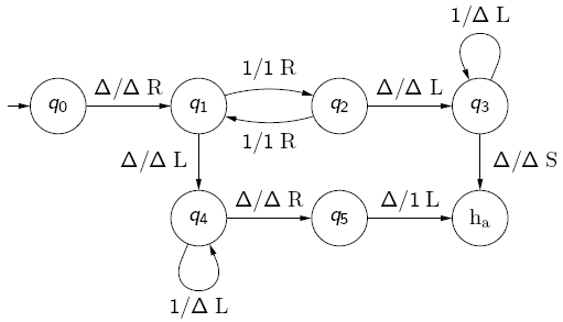
For example, for the following Turing machine, where Σ = {a, b} and Γ = {a, b, Δ}:

Suppose q = q₁, a = a₁ and b = a₂, then we can encode this as e(M) = 00100011000100010100010100011..., which can be broken down as:

001	00011	0001	0001	01	0001	01	00011
s(a)	s(b)	s(q)	s(q)	s(Δ)	s(q)	s(Δ)	s(R)
input alphabet		initial state	transitions

Tape symbols are states are implicit in the transitions, and therefore do not need to be explicitly defined. With this, you can feed the encoding machine into another machine (this is a similar concept to how compilers work).

The Self-Accepting Language

You can define the self-accepting language SA ⊆ {0, 1}* by SA = {w | w = e(M) for some Turing machine M and w ∈ L(M)}. This is basically saying that w is a code of a TM that accepts its own encoding. As such, we can define the completment of SA, SA = NSA = {w ∈ {0, 1}* | w ≠ e(M) ∀ Turing machines M} ∪ {w ∈ {0, 1}* | w = e(M) for some Turing machine M and w ∉ L(M)} - that is, a bit string that does not represent a TM, and a TM that doesn't accept itself.

We have two theorems about the self-accepting language:

SA is recursively enumerable, but not decidable
NSA is not recursively enumerable

Proof of Theorem 2

This is done by contradiction (indirect proof), or reducio ad absurdum and relies on the principle of tertium non dafur. If we suppose that NSA is recursively enumerable, then there is a Turing machine that accepts NSA (for Turing machine M, L(M) = NSA). If we consider the code e(M), then we have two cases:

e(M) ∈ L(M). Then, by assumption, e(M) ∈ NSA. But then, by definition of NSA, e(M) ∉ L(M). This is obviously a contradiction.
e(M) ∉ L(M). Then, by definition of NSA, e(M) ∈ NSA, hence by assumption e(M) ∈ L(M). This is again a contradiction.

It therefore follows that our assumption must be wrong. That is, NSA is not recursively enumerable.

The corollary of this is that SA is not decidable, and the proof of this is by definition of a decidable languages - "If a language is decidable, L is also decidable". As NSA is not r.e., it is not decidable, therefore SA is not decidable.

Proof of Theorem 1

The corollary of the proof from theorem 2 is that SA is not decidable, and the proof of this is by definition of a decidable languages - "If a language is decidable, L is also decidable". As NSA is not r.e., it is not decidable, therefore SA is not decidable.

We also need to consider the theorem that SA is recursively enumerable. To prove this, we need to consider a Turing machine T_SA accepts SA by working as follows:

T_SA first checks that its input w is the code of some Turing machine M (i.e., w = e(M)) and then Σ(M) includes {0, 1}. if this is not the case, T_SA rejects w. Otherwise, T_SA computes e(w) = e(e(M)) and runs U (the universal Turing machine) on e(M)e(w). It follows that T_SA accepts w if and only if M accepts w. Hence L(T_SA) = SA.

The Universal Turing Machine

The universal Turing machine is basically a Turing machine interpreter. It takes inputs of the form e(M)e(w), where M is a Turing machine and w is a string over Σ(M)*. The universal Turing machine will run machine M on input w, and accepts e(M)e(w) if w ∈ L(M) (M accepts w), rejects e(M)e(w) if w ∉ L(M) (M rejects w) and e(M)e(w) loops when M loops on w.

Most Languages are not Recursively Enumerable

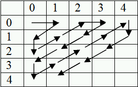
A set S is countably infinite is there exists a bijective function N → S and is countable if it is countably infinite or finite. e.g., countable sets, N, Z, N × N and uncountable sets: R, 2^N

Cantor said that if you plot a matrix of pairs of numbers, and move diagonally you can represent any number with a bijective function, so pairs of numbers are countably infinite, as long as the base number is.

Lemmas:

If S₀, S₁, ... are countable, then S = ∪^∞_{i = 0}S_{i is countable}
If S is an infinite set, then its power set 2^S is uncountable
If S is uncountable, and T is a countable subset of S, then S - T is uncountable

Proof of lemma 2: Let S be countably infinite, as otherwise 2^S is obviously uncountable (there are uncountably many singleton subsets). We proceed by contradiction. Suppose 2^S is countably infinite, then there is an infinite listing S₀, S₁, ... of the elements of 2^S (i.e., of all the subsets of S). Since S is countably infinite, there is a bijection ƒ: N → S. We can define some subset of S as S′ by S′ = {ƒ(i) | i ≥ 0 ^ ƒ(i) ∉ S_i}. Since S′ ⊆ S, there is some n such that S′ = S_n. We can consider two cases:

ƒ(n) ∈ S_n, then ƒ(n) ∉ S′ = S_n, which is a contradiction
ƒ(n) ∉ S_n, then ƒ(n) ∈ S′ = S_n, which is again a contradiction.

Theorem: For every nonempty alphabet Σ, there are uncountably many languages over Σ that are not recursively enumerable.

Proof: Every recursively enumerable language is accepted by some Turing machine. Since Turing machines can be encoded as strings over {0, 1} and {0, 1}* is countably infinite, the set of all Turing machines over Σ is countable as well (every subset of a countable set is countable). Hence, the set of all recusively enumerable languages over Σ is countable too. But, 2^Σ*, the set of all languages over Σ is uncountable by lemma 2, thus by lemma 3: 2^Σ* - {L ⊆ Σ* | L is r.e.} is uncountable as well.

Turing-computable Functions

A Turing machine M = (Q, Σ, Γ, q₀, δ) computes the partial function ƒ_m(x) = {y if (q₀, Δx) ├* (h_a, Δy), undefined otherwise} - which says that ƒ_m(x) = the resulting string on the tape if it halts, otherwise it is undefined. We can generally change this unary function into a k-ary function by saying that M computes for every k ≥ 1. The k-ary partial function ƒ_m : (Σ*)^k → Σ* is defined by ƒ_m(x₁, ..., x_k) = {y, if (q₀, Δx₁Δs₂...Δx_k) ├* (h_a, Δy), undefined otherwise}.

A partial function ƒ : (Σ*)^k → Σ* is Turing computable if there exists a Turing machine M such that ƒ_m = ƒ

Computing Numeric Functions

A partial function ƒ : N^k → N on natural numbers is computable if the corresponding function ({1}*)^k → {1}* is computable, where each n ∈ N is represented by 1ⁿ.

e.g., you could have a Turing machine computing ƒ : N → N with ƒ(x) = if x is even then 1 else 0, which could be represented as

Characteristic Function of a Language

For every alphabet Σ, fix to distinct strings w₁, w₂ ∈ Σ*. The characteristic function of a language L ⊆ Σ* is the total function X_L : Σ* → Σ*, defined by X_L = {w₁ if x ∈ L, w₂ otherwise.

Theorem: A language is decidable if and only if its characteristic function X_L is computable.

Graph of a Partial Function

The graph of a partial function ƒ : Σ* → Σ* is the set, Graph(ƒ) = {(v, w) ∈ Σ* × Σ* | ƒ(v) = w}. This can be turned into a language over Σ ∪ {#}: Graph_#(ƒ) = {v#w | (v, w) ∈ Graph(ƒ)}

We can have two theorems from this:

A partial function ƒ : Σ* → Σ* is computable if and only if Graph_#(ƒ) is recursively enumerable.
A total function ƒ : Σ* → Σ* is computable if and only if Graph_#(ƒ) is decidable.

Decision Problems

A decision problem is a set of questions, each of which has the answer yes or no.

We can say that these questions are instances of the decision problem; depending on their answers, they are either 'yes'-instances or 'no'-instances. To solve decision problems by Turing machines, instances are encoded as strings.

A decision problem P is decidable, or solvable, if its language of encoded 'yes'-instances is decidable. Otherwise, P is undecidable or unsolvable.

A decision problem P is semi-decidable if its language of encoded 'yes'-instances is recursively enumerable.

The Membership Problem for Regular Languages

Input: A regular expression r and w ∈ Σ*
Question: Is w ∈ L(r)
Problem: {(r, w) | r is a regular expression, w ∈ Σ*}
'Yes'-instances: {(r, w) | r is a regular expression and w ∈ L(r)
Encoded 'Yes'-instances: {encode(r)encode(w) | r is a regular expression and w ∈ L(r)}

This problem is decidable, as it can be turned into an automata.

The Self-Accepting Problem

Input: A Turing machine M
Question: Does M accept e(M)?
Problem: {M | M is a Turing machine}
'Yes'-instances: {M | M is a Turing machine and e(M) ∈ L(M)}
Encoded 'Yes'-instances: {e(M) | M is a Turing machine and e(M) ∈ L(M)}

The encoded 'Yes'-instances is the language SA, which is recursively enumerable (L(SA) can be enumerated), but not decidable, therefore this problem is semi-decidable.

The Membership Problem for Recursively Enumerable Languages

Input: A Turing machine M and w ∈ Σ*
Question: Is w ∈ L(M)?
Problem: {(M, w) | M is a Turing machine and w ∈ Σ*}
'Yes'-instances: {(M, w) | M is a Turing machine and w ∈ L(M)}
Encoded 'Yes'-instances: {e(M)e(w) | M is a Turing machine and w ∈ L(M)}

The encoded 'Yes'-instances is MP, the membership problem.

Theorem: The membership problem for recursively enumerable languages is undecidable, but semi-decidable.

Proof: We reduce the self accepting problem (SA) to the membership problem for recursively enumerable languages (MP). That is, we show that if MP is decidable, then SA is also decidable. Since SA was proved to be undecidable, MP must be undecidable too.

Suppose that MP is decidable. Then L(MP) is decidable, i.e., there is a Turing machine T that terminates for all inputs and accepts MP. We can construct a Turing machine T′ that decides SA as follows: T′ transforms its input e(M) into e(M)e(e(M)) (where e(M) = w and is placed in e(M)e(w)). T then starts on this string. This can be represented diagramatically:

T′ terminates for all inputs because T always terminates. Moreover, T′ accepts e(M) if and only if T accepts e(M)e(e(M)), that is, T′ accepts e(M) if and only if e(M) ∈ L(M).

Hence, T′ decides SA, therefore, if we can solve MP, we can solve SA. But, as SA was proved to be undecidable, this is a contradiction. Hence, our assumption that MP is decidable is false, i.e., MP is undecidable.

We can summarise this as: reduction of SA to MP - "If we can solve MP, we can also solve SA" ⇔ "SA is not more difficult than MP" ⇔ "MP is at least as difficult as SA"

Reducing Languages and Decision Problems

Let L₁, L₂ ⊆ Σ* be languages. L₁ is reducible to L₂ if there is a computable total function (i.e., there exists a Turing machine) ƒ : Σ* → Σ* such that for all x ∈ Σ*, x ∈ L₁ if and only if ƒ(x) ∈ L₂.

Let P₁, P₂ be decision problems and e(P₁), e(P₂) be the associated languages of the encoded 'Yes'-instances. We say that P₁ is reducible to P₂ if e(P₁) is reducible to e(P₂).

Theorem 1: Let L₁, L₂ be languages such that L₁ is reducible to L₂. If L₂ is decidable, so is L₁.

Theorem 2: Let P₁, P₂ be decision problems such that P₁ is reducible to P₂. If P₂ is decidable, so is P₁.

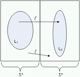
This diagram shows that the strings in L₁ are mapped directly to strings in L₂, and strings in L₁ are mapped to strings in L₂.

L₁ = SA = {e(M) | M is a Turing machine and e(M) ∈ L(M)} and L₂ = MP = {e(M)e(w) | M is a Turing machine and w ∈ w ∈ L(M)}. ƒ : {0, 1}* → {0, 1}* with ƒ(x) = {xe(x) if x = e(M) for some Turing machine M, Λ otherwise.

Halting Problem

Input: A Turing machine M and a string w
Question: Does M reach a halting configuration on input w?
Theorem: The halting problem is undecidable, but semi-decidable

We reduce the membership problem for recursively enumerable languages (MP) to the halting problem (HP). Suppose that HP is decidable, then there is a TM T_halt that terminates on all inputs and accepts an input e(M)e(w) if and only if M reaches a halting configuration (terminates on input w).

We can construct a Turing machine T′ diagramatically as follows:

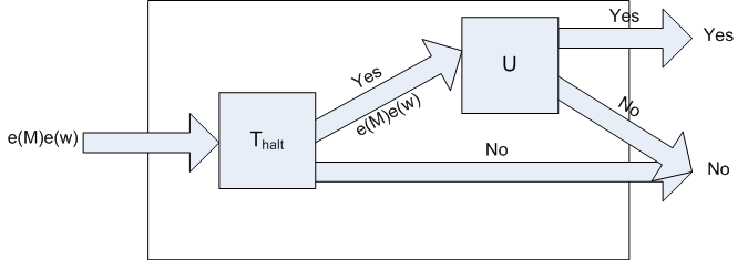
Note that if T_halt outputs 'yes' then U will terminate on e(M)e(w) with either Yes or No. Hence, T′ solves MP. Since MP is undecidable, our assumption that HP is decidable must be false.

Accept_#

Theorem: The following problem (Accept_#) is undecidable.

Input: A Turing machine M such that # ∈ Σ
Question: Is # ∈ L(M)

Proof: We reduce MP to Accept_#. Suppose Accept_# is decidable, then there is a Turing machine that halts on all inputs, accepting input e(M) if and only if # ∈ L(M). We can construct a Turing machine T′ as follows:

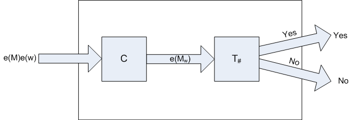
Where C is a Turing machine that transforms e(M)e(w) into the output e(M_w), where M_w is a Turing machine that ignores its input and runs M on input w. Now, T′ solves MP. We can consider two cases:

Case 1: w ∈ L(M). Then, by construction of M_w, M_w accepts every input and hence # ∈ L(M_w), thus T_# accepts e(M_w) and T′ accepts e(M)e(w).

Case 2: w ∉ L(M). Then, by construction of M_w, M_w accepts no input and hence # ∉ L(M_w), this T_# rejects e(M_w) and T′ rejects e(M)e(w).

Since MP is undecidable, Accept_# must be undecidable as well.

Rice's Theorem (1953)

Let C be a proper, non-empty subset of all recursively enumerable languages. Then, the following problem is undecidable:

Input: A Turing machine M
Question: Is L(M) ∈ C?

In other words, every nontrivial property of recursively enumerable languages is undecidable. A property is nontrivial if it is satisfied by a proper, nonempty subset C of the class of all recursively enumerable languages. e.g., for the problem "Is L(M) finite?" C = {L = Σ* | L is finite}

Beware, Rice's theorem is about the languages accepted by Turing machines, not about the machines themselves.

Undecidable Problems About Context Free Grammars

Input: A context free grammar G
Question: Is L(G) = Σ*

Input: Two context free grammars G₁ and G₂
Question: Is L(G₁) = L(G₂)

Input: Two context free grammars G₁ and G₂
Question: Is L(G₁) ∩ L(G₂) = ∅?

Input: A context-free grammar G
Question: Is G ambiguous?

Input: A context-free grammar G
Question: Is L(G) inherently ambiguous?

In all the cases above, apart from the question 'Is G ambiguous?', the CFGs can be replaced by pushdown automata. However, in the case of 'Is G ambiguous?', this refers to a property of a grammar, not a language, so a pushdown automata can not be substituted in.

The Church-Turing Thesis

The Church-Turing thesis was proposed by Alonzo Church and Alan Turing in 1936 and is the statement that "Every effective procedure can be carried out by a Turing machine".

A functional version of this statement is that every partial function computable by an effective procedure is Turing-computable, and for decision problems, every decision problem solvable by an effective procedure is decidable.

This is only a thesis as an effective procedure (algorithm) can not be defined.

Complexity

(By convention when dealing with complexity, we only consider Turing machines, both deterministic and nondeterministic of which all computations eventually halt).

The time complexity of a Turing machine M is function τ_M : N → N, where τ_M(n) is the maximum number of transitions M can make on any input of length n. For a nondeterministic Turing machine N, τ_N(n) is the maximum number of transitions N can make on any input of length n by employing any choice of transitions. The time complexity of (possibly nondeterministic) multitape machines is defined analogously, and we define the time complexity as above as the worst-case complexity.

The space complexity of a Turing machine M is the function s_M : N → N, where s_M(n) is the maximum number of tape squares M visits on any input of length n. For a nondeterministic Turing machine N, s_N(n) is the maximum number of tape squares N visits on any input of length n by employing any choice of transitions. For multitape Turing machines, the maximum number of tape squares refers to the maximum of the numbers for the individual tapes (which differs only be a constant factor from the maximal number of squares visited on all tapes altogether).

For every Turing machine M, s_M(n) ≤ τ_M(n) + 1, as it is impossible for more squares to be visited than transitions made.

Growth Rate of Functions

Given a function f, g : N → N, f is of order g, written as f = Ο(g), or f ∈ Ο(g), if there is c, n₀ such that ƒ(n) ≤ c . g(n) ∀ n ≥ n₀.

Theorem, for a, b, r ∈ N with a, b > 1

log_a(n) = Ο(n) but n ≠ Ο(log_a(n))
n^r = Ο(bⁿ) but bⁿ ≠ Ο(n^r)
bⁿ = Ο(n!) but n! ≠ Ο(bⁿ)

Using this 'Big-O' notation, we can create a hierarchy of complexity:

Name	Ο
Constant	1
Logarithmic	log n
Linear	n
Log-linear	n log n
Quadratic	n²
Cubic	n³
Polynomial	n^p
Exponential	bⁿ
Factorial	∞

The table below shows examples of different growth rates for different values of n.

log₂(n)	n	n²	n³	2ⁿ	n!
2	5	25	125	32	120
3	10	100	1000	1024	3628800
4	20	400	8000	1048576	2.4 × 10¹⁴
5	50	2500	125000	1.1 × 10¹⁵	3.0 × 10⁶⁴
6	100	10000	1000000	1.2 × 10³⁰	> 10¹⁵⁷

Properties of Time Complexity

Theorem - multiple tapes vs. one tape: For every k-tape Turing machine M there is Turing machine M′ such that L(M′) = L(M) and τ_M′ = Ο(τ_M²).

Theorem - there are aribtrarily complex languages. Let ƒ be a total computable function. Then there is a decidable language L such that for every Turing machine M accepting L, τ_M is not bounded by ƒ.

Theorem - there need not exist a best Turing machine. There is a decidable language L such that for every Turing machine M accepting L, there is a Turing machine M′ such that L(M′) = L(M) and τ_M′ = Ο(log(τ_M)).

The Classes P and PSpace

A language L is recognisable in polynomial time if there is a deterministic Turing machine M accepting L such that τ_M = Ο(n^r) for some r ∈ N. The class of all languages recognisable in polynomial time is denoted by P.

A language L is recognisable in polynomial space if there is a deterministic Turing machine M accepting L such that s_M = Ο(n^r) for some r ∈ N. The class of all languages recognisable in polynomial space is denoted by PSpace.

A decision problem is said to be in P resp. PSpace if its language of encoded 'yes'-instances is in P resp. PSpace.

The Classes NP and NPSpace

A language L is recognisable in nondeterministic polynomial time if there is a nondeterministic Turing machine N accepting L such that Τ_N = Ο(n^r), for some r ∈ N. The class of all languages recognisable in nondeterministic polynomial time is denoted by NP.

A language L is recognisable in nondeterministic polynomial space if there is a nondeterministic Turing machine N accepting L such that s_N = Ο(n^r) for some r ∈ N. The class of all languages recognisable in nondeterministic polynomial space is denoted by NPSpace.

A decision problem is said to be in NP resp. NPSpace if its language of encoded 'yes'-instances is in NP resp. NPSpace.

Example: A problem in P

A graph G = (V, E) consists of a finite set, V, of vertices (or nodes) and a finite set, E, of edges such that each edge is an unordered pair of nodes. A path is a sequence of nodes connected by edges. A complete graph (or clique) is a graph where each two nodes are connected by an edge.

The path problem has input of a graph G and nodes s and t in G and the question does G have a path from s to t?

The theorem is that the path problem is in P, and the proof for this is the following algorithm which solves the path problem:

On input (G, s, t) where G = (V, E) is a graph with nodes s and t:

Mark node s
Repeat until no additional nodes are marked
1. scan all edges of G
2. for each edge {v, v′} such that v is marked and v′ is unmarked, mark v.
Check if t is marked - accept, otherwise reject

The running time of this algorithm can be considered by considering each stage. Stages 1 and 3 are considered only once. The body of the loop in stage 2 is executed at most |V| times, because each time except for the last, an unmarked node is marked. The body of the loop can be executed in time linear in |E| and stages 1 and 3 need only constant time. Hence, the overall running time is Ο(|V| × |E|). In the worst case, |E| = |V|²/2, and hence in Ο(|V|³).

Example: Problems in NP

The complete subgraph (clique) problem has the input of a graph G and k ≥ 1. The question is does G have a complete subgraph with k vertices?

The Hamiltonian circuit problem takes an input of a graph G, and the question is does G have a Hamiltonian circuit (a path v₀, ..., v_n through all nodes of G such that v₀ = v_n and v₁, ..., v_n are pairwise distinct.

Theorem: The complete subgraph and the Hamiltonian circuit problems are in NP.

The clique problem can be solved by a nondeterministic Turing machine in polynomial time. N nondeterministically selects ("guesses") vertices v₁, ..., v_k in G and checks whether each pair {v_i, v_j}, 1 ≤ i ≤ j ≤ k is an edge in G. This checking can be done in time polynomial in |V| + k.

G can be represented as a string of vertices followed by a string of edges in the form of vertex pairs. Then, at most k²/2 vertex pairs have to be checked, which can be done in time |V|²/2 × k²/2.

Tractable Languages

A language is tractable if L ∈ P, otherwise L is intractable.

A language L is recognisable in exponential time if there is a Turing machine M accepting L such that τ_M = Ο(2^{n^r}) for some r ∈ N. The class of all languages recognisable in exponential time is denoted by ExpTime.

Theorem:

P ⊆ NP ⊆ PSpace = NPSpace ⊆ ExpTime
P ≠ ExpTime

There is an open research problem of does P = NP.

Conjectured Hierarchy of Complexity Classes

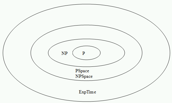
(Only P ≠ ExpTime is known, but it is not known whether the other subsets above are proper or not)

Inclusions P ⊆ NP and PSpace ⊆ NPSpace, as every deterministic Turing machine can be represented by a nondeterministic Turing machine.

Inclusions P ⊆ PSpace and NP ⊆ NPSpace, as every Turing machine (deterministic or nondeterministic) satisfies s_M(n) ≤ τ_M(n) + 1, as we can not visit more squares than we can do transitions. Hence τ_M = Ο(n^r) implies s_M = Ο(n^r).

Inclusions NPSpace ⊆ PSpace. This can be proved using Savitch's Theorem (which is nontrivial), which states that for every nondeterministic Turing machine N there is a Turing machine M such that L(M) = L(N) and s_M = s_N², and a polynomial squared is still a polynomial.

Inclusions PSpace ⊆ ExpTime. For an input of length n each configuration of the Turing machine M can be written as follows: (q, a₀...a_i...a_{s_M(n)}). For each part, there are |Q| possible states, s_M(n) possible tape head positons and |Γ|^s_M(n) possible tape content configurations. Hence, the maximum number of configurations is |Q| × s_m(n) × |Γ|^s_M(n) = Ο(Γ|^s_M.

A Turing machine computation that halts does not repeat any configurations. Hence τ_M = Ο(k^s_M for some k, and it follows our inclusion, hence PSpace ⊆ ExpTime (for k ≤ 2^m we have k^{n^r} ≤ (2^m)^{n^r} = 2^{mn^r} = 2^{n^{m + r}}).

Polynomial-time Reductions

A function ƒ is polynomial-time computable if there is a Turing machine M with τ_M = Ο(n^r) that computes ƒ.

Let L₁, L₂ ⊆ Σ* be languages. L₁ is polynomial-time reducible to L₂ if there is a polynomial-time computable total function ƒ : Σ* → Σ* such that for all x ∈ Σ*, x ∈ L₁ if and only if ƒ(x) ∈ L₂.

Theorem: Let L₁ be polynomial-time reducible to L₂. Then: L₂ ∈ P implies L₁ ∈ P; L₂ ∈ NP implies L₁ ∈ NP.

Proof

Since L₂ ∈ P there is a Turing machine M₂ with polynomial time complexity that decides L₂. Moreover, since L₁ is polynomial-time reducible to L₂, there is a Turing machine M with polynomial-time complexity such that ƒ_M : Σ* → Σ* satisfies for all x ∈ Σ*, x ∈ L₁ if and only if ƒ_M(x) ∈ L₂.

Let M₁ be the composite Turing machine MM₂ which first runs M and then runs M₂ on the output of M, then L(M₁) = L₁.

Since |ƒ_M(x)| can not exceed max(τ_M(|x|), |x|), the number of transitions of M₁ is bounded by the sum of the following estimates of the seperate computations:

(a) τ_M₁(n) ≤ τ_M(n) + τ_M₂(max(τ_M(n), n))

Let τ_M = Ο(n^r), then there are constants c and n₀ with τ_M(n) ≤ c . n^r ∀ n ≥ n₀.

Let τ_M₂ = Ο(n^t), then there are constants c₂ and n₂ with τ_M₂(n) ≤ c₂ . n^t ∀ n ≥ n₂.

Hence τ_M₂(n) ≤ c₂.n^t + d₂, ∀ n ≥ 0, where d₂ = {τ_M₂(k) | k < n₂}.

It follows τ_M₂(τ_M(n)) ≤ c₂ . (τ_M(n))^t + d₂, for all n ≥ 0, and hence τ_M₂(τ_M(n)) ≤ c₂ . (c . n^r)^t + d₂, for all n ≥ 0

So, τ_M₂(τ_M(n)) ≤ c₂c^t . n^rt + d₂ ∀ n ≥ 0.

Thus, by formula (a) above, τ_M₁ = Ο(n^rt), hence L₁ ∈ P (r and t are constants, therefore n^rt ∈ P)

Hardness

If L₁ is polynomial-time reducible to L₂, then L₁ is no harder than L₂. Equivalently, L₂ is at least as hard as L₁.

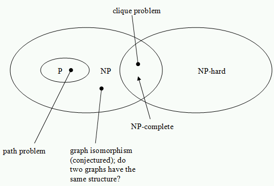
A language L is NP-hard if every language in NP is polynomial-time reducible to L; A NP-hard language is at least as hard to decide as every language in NP. Equivalently, no language in NP is harder to decide than any NP-hard language.

A language L is NP-complete if it is NP-hard and belongs to NP; a NP-complete language is a "hardest" language in NP. Corollary, for every NP-complete language L, L ∈ P if and only if P = NP.

Assuming P ≠ NP:

The Satisifability Problem

Consider boolean expressions built from variables x_i and connectives ^, ∨ and ¬. A literal is either a variable x_i, or a negated variable ¬x_i. An expression C₁ ^ C₂ ^ ... ^ C_n is in conjunctive normal form (CNF) if C₁, ..., C_n are disjunction of literals.

An expression C is satisfiable if there is an assignment of truth values to variables that make C true.

e.g., C = (x₁ ∨ x₃) ^ (¬x₁ ∨ x₂ ∨ x₄) ^ ¬x₂ ^ ¬x₄. In this case, C is satisfiable by the assignment α = {x₁, x₂, x₄ → false, x₃ → true}

The satisfiability problem takes input of a boolean expression C in CNF, and the question is "Is C satisfiable?".

Theorem: The satisfiability problem is NP-complete. This was proved by S. A. Cook in 1971 was was the first problem to be shown to be NP-complete.

To prove a problem is NP-complete, any NP-complete problem should be reducible to it. e.g., a polynomial-time reduction of the satisfiability problem to the clique problem. What we need is a function ƒ : x → (G_x, k_x), where x if a CNF expression and (G_x, k_x) is a pair depending on x, such that x is satisfiable if and only if G_x has a clique with k_x vertices.

Let x = ^^c_{i = 1}∨^d_i_{j = 1}a_{i, j}, where ^ and ∨ are conjuncts and each a_{i, j} is a literal.

Observation: Pick one literal from each conjunct and connect each pair of picked literals that is not complimentary (e.g., x and ¬x are complimentary). If this yields a complete graph, then x is satisfiable. Vice versa, if x is satisfiable, then a complete subgraph can be constructed in this way.

Idea: Choose G_x as the graph consisting of all occurences of literals and all connections between literals that are in different conjuncts and not complimentary.

Define G_x = (V_x, E_x) by V_x = {(i, j) | 1 ≤ i ≤ c ^ 1 ≤ j ≤ d_i} and E_x = {((i, j), (l, m)) | i ≠ l ^ a_{i, j} ¬≡ ¬a_{l, m}}, and let k_x = c.

By construction of G_x: Two vertices are linked if and only if their literals are in different conjuncts and there is a truth assignment making both literals true. Next, we show that ƒ is a reduction from the satisfiability problem to the clique problem.

"Only if": Let x be satisfiable. Then there is a truth assignment α such that for each i, there is some literal a_i, j_i with α(a_i, j_i) = true. Hence, by construction of E_x, the vertices (1, j₁), (2, j₂), ..., (k_x, j_{k_x}) forms a clique in G_x. Note that a_{i, j_i} ¬≡ ¬a_{i, j_i}, because α(a_i, j_i) = true = α(a_{i, j_i}).

"If": Let G_x have a clique with k_x many vertices. Then, by definition of E_x, the literals of these vertices must be pairwise non-complimentary. Hence, there is a truth assignemtn Θ making all of these literals true. Moreover, by the definition of E_x, these k_x literals are in k_x different conjuncts. So α makes each of the k_x = c conjuncts true. Thus, x is satisfiable.

Context-Sensitive Languages

Linear Bounded Automata

Turing Machines

Configurations and Transitions

Non-deterministic Turing Machines

Multi-tape Turing Machines

Recursively Enumerable

Enumerating Languages

Computability

Decidability

Theorem:

Proof of Theorem 2

Proof of Theorem 3

Encoding Turing Machines

The Self-Accepting Language

Proof of Theorem 2

Proof of Theorem 1

The Universal Turing Machine

Most Languages are not Recursively Enumerable

Turing-computable Functions

Computing Numeric Functions

Characteristic Function of a Language

Graph of a Partial Function

Decision Problems

The Membership Problem for Regular Languages

The Self-Accepting Problem

The Membership Problem for Recursively Enumerable Languages

Reducing Languages and Decision Problems

Halting Problem

Accept#

More Undecidable Problems

Rice's Theorem (1953)

Undecidable Problems About Context Free Grammars

The Church-Turing Thesis

Complexity

Growth Rate of Functions

Properties of Time Complexity

The Classes P and PSpace

The Classes NP and NPSpace

Example: A problem in P

Example: Problems in NP

Tractable Languages

Conjectured Hierarchy of Complexity Classes

Polynomial-time Reductions

Proof

Hardness

The Satisifability Problem

Accept_#