Natural Language Processing

The ultimate goal of NLP is to build machines that can understand human language, using speech and language processing.

At present and in the near future, NLP can used for information extraction (robust, large-scale shallow NLP for automated shallow understanding, e.g., e-mail scanning, CV processing, database extraction, etc), language based interaction with everyday devices, domain specific information systems (such as call centres with question/answering systems), and to aid the aged and disabled (responding to emergency situations, being used for long-term health monitoring, or for companionship and entertainment).

NLP is hard due to ambiguity in natural languages, whether phonetic (I scream vs. ice cream) at the lowest level, syntactic, semantic, or pragmatic (different contexts give different semantic meanings) at the highest level.

Natural language understanding systems go through many stages. e.g., a virtual agent system starting with the user query and ending with an engaging response has:

A spelling corrector;
A tagger (which disambiguates syntactic words and performs lexical scanning, e.g., tagging things as nouns, adjectives, verbs, etc);
A chunker/parser;
A phrase matcher;
A dialog engine (which feeds back into the matcher);
A gesture planner (for an on-screen character - the gesture comes from the class of word, e.g., if it's a happy work, the previous mood, and the personality of the character, i.e., how often the mood changes);
An animation client.

A more general version of the NLP pipeline starts with speech processing, morphological analysis, syntactical analysis, semantic analysis, applying pragmatics, finally resulting in a meaning.

Spelling Correction

Spelling errors are common in written user queries, and the types of errors can be classified:

Insertions (e.g., beinefits);
Deletions (e.g., benfits);
Transposititons (e.g., bneefits);
Repetitions (e.g., bennefits);
Replacements (e.g., benifits).

A simple technique to detect which word a misspelt word is supposed to be is edit distance (that is, number of errors of the types above a candidate word is from the misspelt word).

This method only corrects single errors, but can be extended to multi-error cases.

The probabilities are estimated from real data, so therefore incorporate domain data automatically. If there are two ways to get to a word, then their probabilities are combined.

Robust Parsing

In addition to spelling correction, two issues for robust natural language understanding include robust parsing (dealing with unknown or ambiguous words) and robust semantic tagging.

Robust parsing must consider the two stages of parsing: part-of-speech (PoS) tagging and syntactic parsing (both shallow and deep).

PoS tagging is the pre-step to syntactic analysis - it tags words with their type, e.g., pronoun, verb, noun, etc, but at this level there can be ambiguity and unknown words. The goal is to assign the correct PoS tags.

One way to solve this is to construct canonical logical forms from sentences (e.g., the following are roughly equivalent: "John bought a toy" and "A toy was bought by John").

Context free grammars are deficient in many ways for dealing with ambiguity, and can not handle common phenomena such as relative clauses, questions or verbs which change control.

Structural ambiguity, such as propositional phrase (PP) attachment ambiguity, where attachment preference depends on semantics (e.g., "I ate pizza with ham" vs. "I ate pizza with my hands"). Current systems are not very accurate at dealing with this (~74%), so it is often better to leave PPs unattached rather than guessing wrong. Position-based and meaning-based matching can be used to combat this.

For semantic tagging, we must also deal with robustness in the named entity recognition and sense disambiguation phases. For named entity recognition, this deals with open class words such as person, location, date or time or organisation names. Known words are left to a later stage.

Word sense disambiguation is still difficult. The most frequent WordNet sense baseline gives ~64%, and the best supervised systems achieve ~66-70%, with unsupervised systems achieve ~62%. Question and answer systems can do without full sense disambiguation though.

Morphology

Morphology is the study of the structure within words.

Morphemes are the smallest grammatical unit, and can be free (which are words of their own right), or bound (where they can only exist as part of other words, e.g., prefixations and suffixations in English).

Inflectional morphology is used to get different forms of a verb or noun. They are functional (in that the affix acts like a function e.g., suffix s on nouns always gives a plural form), productive (new words conform to the rules) and preserve category (the major category, e.g., noun/verb is not changed).

Derivational morphology is used to get new words from existing stems (e.g., national from nation+al). It is relational (adding the same suffix to two different stems can have different semantic effects), partly productive (some are in current use, whereas others are historic relics) and alters the category (e.g., national (adj) vs. nation (n)).

Morphological analysis typically uses just inflectional morphology, mainly as it is too impractical to store the entire lexicon (which is too large, and can not deal with unknown words), so our lexical lookup involves morphological analysis, so a word is a base form and affixes/inflection.

Morphological analysis is non-trivial, as we can not assume, for example, that re- is a prefix for all words, e.g., read is not re+ad. Our morphological analysis process takes 3 steps:

Segment the word into stem + affix, e.g., walked → walk+ed, bought → buy+ed (this case is more difficult);
Lookup the grammatical category for the stem, e.g., walk → verb, base;
Apply the inflection rule for +ed, e.g., (verb, base) → (verb, psp).

Inductive Logic Programming

Inductive logic programming (ILP) is a symbolic machine learning framework, where logic programs are learnt from training examples, usually consisting of positive and negative examples. The generalisation and specialiation hierarchy of logic programs is exploited.

Morphological analysis
slide 11

In Prolog, _ is more general than (X, _), which in turn is more general than (X, Y).

For morphological learning, all base forms cover some positive examples, but no negative examples.

First-order decision lists are essentially Prolog representation for functions. Every clause is terminated by !, the cut operator. This tells Prolog to stop searching as soon as the cut is reached, and therefore only get the first solution (and is therefore a function).

These can also be thought of as ordered classes, with the specific clauses at the top and the general clauses at the bottom.

For morphology learning, we have training examples consisting of (baseform, inflected_form) and the task to learn rules that predict inflected form given a base form, and a base form given an inflected form. However, we must also consider the negative examples. Fortunately, these are implicit, as if (likes, like+s) is a positive example, than the following negative examples exist: (likes, lik+es), (likes, li+kes), etc. This is due to it being typically sufficient to assume that functions are being learnt, and recall the universal property of functions, that for any input x, ƒ(x) is unique.

Another form of learning is called bottom-up learning, where we go from examples to clauses. For each example, a generalisation is generated that covers the example, and all such clauses form a generalisation set.

Syntax

Formally, the coverage of a grammar G refers to the set of sentences generated by that grammar, i.e., it is the language generated by that grammar.

In natural language, we say that a grammar overgenerates if it generates ungrammatical sentences, or undergenerates if it does not generate all grammatical sentences. Typically grammars undergenerate, but will also overgenerate to a lesser extent.

However, with natural language, adequacy is a more important concept, that is, how well does the grammar capture the linguistic phenomena? It needs to be adequate for syntactic phenomena to be captured.

In linguistics, grammars are more than just a syntax checking mechanism, they should also provide a recipe for constructing a meaning. Therefore, grammars are needed to assign structure to a sentence in such a way that language universal generalisation are preserved, and language specific generalisations are preserved. Transformations can therefore be defined that relate sentences with related meaning.

We say that grammars allow a productive method for constructing the meaning of a sentence from the meaning of its parts.

Linguistic Universals

The following are assumed to be true for all human languages:

Nouns denote classes of objects, concrete or abstract;
Verbs denote events;
Noun phrases denote objects;
Verb phrases;
Subcategorisation;
Noun modifiers (adjectives);
Verb/sentential modifiers (adverbs);
Relative clauses.

Taking these linguistic views are useful as it allows for easier meaning construction, and should result in better coverage. Ultimately, they will help build natural language understanding systems that port easily across languages.

In addition to these linguistic universals, there are some language specific generalisations, such as in English, where adjectives always precede nouns, and verbs normally precede their objects, or in Japanese and Hindi, where objects precede the verb.

English Grammar

Pronouns are shorthand references to nouns (he, she, it, that, etc).
Adjectives are modifiers for nouns.
Adverbs are modifiers for verbs and sentential expressions (quickly, very, etc).
Auxiliary verbs are used to express tense information (e.g., is - present, was - past, -ing - continuous or progressive).
Modal auxiliaries are used to express possibility, permission, wish, etc (e.g., must, can, may, should, would, shall).

We also have constraints on our grammar such as determiner-noun agreement (singular/plural noun phrases, e.g., these hobbits vs. this hobbit), subject-verb agreement (subjects must agree with the main verb, e.g., John likes tomatoes vs. I like tomatoes) and pronouns, which apply to the person (first person, second person, etc) and the number being referred to (e.g., I, you, he, she, we, they).

Applying these agreements to a context-free grammar result in a lot of rules, a lot of which are roughly the same structure (see Introducing Syntax - slide 23), and this gets worse when you start considering tensed forms of verbs.

Other rules to consider is the case system. Pronouns in English are marked for the nominative and accusative case (e.g., He likes Mary, but not Mary likes he - Mary likes him).

There are also auxiliary verbs, such as the different forms of have and be. We can consider two further factors here: tense and aspect. Tense refers to time (when an event happened) and is usually expressed by the main verb, whereas aspect refers to the duration, completion or repetition, and is usually expressed by an auxiliary verb.

Modal verbs can also be used to express the modality.

In English, there are syntactic constraints on auxiliary verbs. The order, in particular, is fixed. The have auxiliary comes before be, using be/is selects the -ing (present participle) form.

As we can see above, problems with using context-free phrase structure grammars (CF-PSG) include the size they can grow too, an inelegant form of expression, and a poor ability to generalise.

Natural languages are believed to be at least context-free, but there is some evidence they are context-sensitive. Simple natural language phenomena (e.g., NP-NP, V-NP-NP patterns) can be described using regular grammars, but this does not cover all linguistic phenomena, such as relative clauses, so natural languages must be at least context-free.

There is some evidence from Swiss-German and Dutch to suggest that natural languages are not context free - these are known as cross-serial dependencies. However, CFGs are largely sufficient for describing natural languages.

Definite Clause Grammars

Definite clause grammars (DCGs) generalise over context-free grammar rules. A DCG is a CF-PSG except for one difference: non-terminals can be Prolog/first-order terms. This allows us to collapse our CFG to be parameterised and considerably more compact. (see slides 4 and 5 in the DCG notes for an example).

However, DCGs are more powerful than CFGs, and rules such as s --> np(A,B), vp(A,B) could have infinite instantiations. However, DCGs have a CFG backbone, and if we restrict the arguments for a DCG, we get the CFG power.

DCGs in Prolog

Prolog supports the syntactic sugar -->, so that the following are equivalent: s --> np, vp. and s(S) :- np(S1), vp(S2), append(S1, S2, S)., and np --> [john]. becomes np([john])..

This sugar defines a top-down depth-first parser, and exploits the top-down depth-first Prolog interpreter.

Using Prolog's difference lists, we can simply do something like: s(S1-S3) :- np(S1-S2), vp(S2-S3)., or for terminals: np([john|X]-X).

However, the actual implementation is a bit different, as s(S1-S3) is actually represented as s(S1,S3), similarly for lexical entries. They are essentially equivalent, however.

Modifiers are used to modify the meaning of a head (e.g., noun or verb) in a systematic way. In other words, modifiers are functions that map the meaning of the head to another meaning in a predictable manner. e.g., book on the table ( book(x) & on(x, y) & table(y) ) to book on the table near the sofa ( book(x) & on(x, y) & (table(y) & near(y, z) & sofa(z)) ).

Usually, modifiers only further specialise the meaning of the verb/noun and do not alter the basic meaning of the head. For a modifier to apply, the head must be compatible semantically. Modifiers can be repeated, successively modifying the meaning of the head (e.g., book on the box on the table near the sofa).

The interpretation of complements is totally determined by the head, and the number of complements a head can take is also determined by the head (e.g., king of France vs. picture of Jim - in both cases, the meaning of of is determined by the head, and it is different in both cases).

Complements can not be repeated without turning them into modifiers. In sentences where both modification and complementation are possible, then world or pragmatic knowledge will dictate the preferred interpretation. When there is not strong pragmatic preference for either readings, then complementation would be preferred.

Proposition phrases (PPs) are usually ambiguous in English, e.g., "I saw the man with a telescope", and most PPs can be attached to both verbs and nouns.

This attachment preference is pragmatic (e.g., I ate pizza with chips vs. I ate pizza with fork), and is difficult for current systems (accuracy is often below 80%).

Propositional verbs are verbs taking propositional (i.e., sentential) arguments, e.g., believe, claim, trust, etc.

Control verbs are used to control the NP argument of a subcategorised VP, e.g., promise is a subject control verb, and persuade an object control verb (contrast "Sandy promised Kim to come home early" vs. "Sandy persuaded Kim to come home early").

Movement occurs when the argument or complement of some head word does not fall in the standard place, but has moved elsewhere. We say that for every space, or gap, where there must be a NP, there is a filler elsewhere in the sentence that replaces it (this is a one-to-one dependency). This gap and filler must have the same category.

There can be an unbounded amount of words and structure between the head word and its moved argument. We can add verbs taking sentential arguments an unbounded number of times, and still maintain a syntactically allowable sentence - this gives us what are known as unbounded dependencies between words.

In order to capture these unbounded dependencies in a grammar, we can use a technique that uses DCGs called "gapping". A sentence with unbounded dependencies has three distinct sections: top (where the filler is), the middle (the structure separating the gap from the filler) and the bottom (where the gap is).

At the top, we add an argument to the nonterminals to indicate whether or not the non-terminal has a gap (i.e., missing NP). Two rules are added to do this. The first rule allows sentences to be built with or without a gap, and marks the S non-terminal with whether or not it has a gap (S(Gap) --> NP VP(Gap)). The second rule takes a sentence that has a gap in it and adds a filler to turn it into a sentence that no longer has a gap (S(nogap) --> NP S(gap)). Complete sentences are now trees rooted by S(nogap).

At the bottom level, gaps must be identified. For transitive verbs, are rules will be: VP(nogap) --> Vt NP and VP(gap) --> Vt.

To complete the picture, the middle must have rules that allow the gap to propagate from the bottom to the top, where it is discharged by the filler. The S rule we had above will deal with some cases, but for VPs, we need VP(Gap) --> Vs S(Gap)m and also for nouns that move: N --> N S(gap).

These simple cases do not deal with semantics however. In the general case, the binding of the semantic value must be retained.

Simple relative clauses can also be handled in a similar way, e.g., NP --> NP S(NP). This is essentially a modifier rule.

Parsing

The task of parsing is defined as enumerating all parses for a given sentence. For any sentence of length n, there are 2ⁿ ways of bracketing them. Bracketing ignores non-terminal assignments on tree nodes. We would therefore expect that the complexity of parsing a CFG is exponential. In reality, even regular grammars are exponential, but recognition can be done in linear time (e.g., with a DFA).

A recogniser gives a yes or no answer for whether a string is allowed by the grammar or not. A parser is a recogniser that also returns a parse tree. Parse trees are used to represent the derivation, and the best representation is as a tree.

A parser should be sound, complete and efficient.

For backtrack parsers, worst-case recognition complexity is exponential. Tabulated parsing avoids recomputation of parses by storing it in a table, known as a chart, or well-formed substring table. In the worst-case, it has n³ complexity.

Tabulated parsing takes advantage of dynamic programming and stores results for a given set of inputs in a table. This is very useful for recursive algorithms.

Top-Down Parsing

Top-down parsers start by proving S, and then rewrite goals until the sentence is reached. Parsers have a choice of which rule to apply, and in which order. DCG parsing in Prolog is top-down, which very little or no bottom-up prediction.

Top-down parsers are sound, but incomplete (top-down, left-to-right, depth-first parsers do not terminate if the grammar contains left-recursive rules) and inefficient (due to the recalculation in backtracking, and if there are lots of different rules with the same LHS.

Bottom-Up Parsing

Bottom-up parsing starts with words, and then matches right-hand sides to derive a left-hand side. It completes when S is derived. The choices a parser has to make are which right-hand side (typically there is less choice here) and the order it is parsed in.

Bottom-up parsers use a method called shift-reduce, consisting of a stack and a buffer.

Bottom-up parsers are sound and complete, but are inefficient in the recalculation in back-tracking, and when there is lexical abiguity.

Left Corner Parsing

Left corners parsing uses the rules, and provides top-down lookahead to a bottom-up parser by pre-building a lookahead table.

For any non-terminals A, B, C, the left-corner relation lc(A, B) is defined as follows:

lc(A, A) - reflexive;
lc(A, B) if A → B … is a CFG rule (immediate left-corner);
if lc(A, B) and lc(B, C) then lc(A, C) - transitive.

This definition is an approximate algorithm. The non-terminals are worked through (in Prolog, this is done using a failure-driven loop).

Bottom-up parsing is used to wait for a complete right-hand side, and then left-corner parsing predicts rules with the right left-corner. It removes many choices.

Left-corner parsing reduces local ambiguity, increases efficiency and increases psychological plausibility.

CKY Algorithm

The CKY, or Cocke-Kasami-Younger algorithm requires grammars to be in Chomsky normal form (i.e., binary branching). The theorem is that for every CFG, there is a weakly equivalent CFG in Chomsky normal form.

A binary function is defined that takes two sets of non-terminals {a₁, …, a_m} and {b₁, …, b_n} and returns {g₁, …, g_p}, such that if α ∈ {a₁, …, a_m} and β ∈ {b₁, …, b_n}, then g ∈ {g₁, …, g_p} if g → αβ.

This function can be implemented efficiently, e.g., by storing the sets as a list of integers. Sentence length does not affect the time complexity of this function.

We also create a matrix of size (n + 1)², which we call the chart. This is initialised such that chart(i - 1, i) = { A | A → word_i }.

The CKY algorithm essentially completes the chart entries by using the following equation: chart(i, j) = ∪_{i < k < j} chart(i, k) × chart(k, j).

To ensure completeness, some control is needed.

for j from 1 to n do

	    chart(j - 1, j) = { A | A → word_k }

	    for i from j - 2 to 0 do

	        for k from i + 1 to j - 1 do

	            chart(i, j) = chart(i, j) ∪ (chart(i, k) × chart(k, j))

	if S ∈ chart(0, n) then return true else return false

The complexity of this algorithm is n³.

CKY is an instance of a passive chart parsing algorithm, i.e., chart entries correspond to completed edges. A disadvantage of bottom-up parsing is that parsing is not sufficiently goal-driven. All subconstituents, whether or not they get incorporated into the final parse, will be found.

Earley Algorithm

CKY parsers have no top-down prediction, work only for Chomsky Normal Form grammars and have no flexible control.

The Earley algorithm is a chart parsing algorithm that works for any CF-PSG. It has an active chart that consists of parse bits, and goals.

The Earley algorithm uses dotted rules, that is, partially completed edges. For the rule vp --> v np, it may exist in three states: vp --> .v np, which is a VP with nothing found, vp --> v .np, which is a VP with a V found, and vp --> v np., which is a complete VP.

Proved and unproved goals are stored, and this is often represented in a chart form.

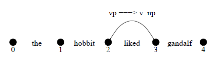
This edge can be written as: ₂vp → v ₃ np.

The Earley algorithm has a fundamental rule: (_iL → α _j X β) × (_jX → γ _k) = (_i L → α X _k β), where α, β is a sequence of NTs, and X is a NT.

In other words, if we have an incomplete edge from i to j (this is the active edge), and a complete edge (that is, where everything has been found) from j to k, then the two can be combined and the active edge extended.

The Earley algorithm also defines two operations: complete, which takes a complete edge and looks left for an active edge to match; and scan, which takes an active edge and looks right for a complete edge to match.

To enter edges, first the algorithm checks an edge is not present, and then predicts either active edges from complete ones (if bottom-up) or active edges from new active ones (top-down). It finishes by completing (combining complete edges to the left) and then scanning (combining active edges to the right).

In bottom-up active chart parsing, the active edge is predicted from complete; when a complete edge is found, rules are predicted that could use it. The rule that defines this is if _i C → α _j is added, then for all rules B → C β, the edge _i B → _i C β is added. This is immediate left corner parsing.

This needs initialisation, so all lexical edges are entered.

Top-down active chart parsing is similar, but the initialisation adds all the S rules at (0,0), and the prediction adds new active edges that look to complete. Now, our predict rule is if edge _i C → α _j X β then for all X → γ, add _j X → _j γ.

Agenda-based Parsing

Agenda-based parsing does not assert new edges immediately, but instead adds them to an agenda or queue. The edges are them removed in some order from the agenda.

A more flexible control of parsing can be achieved by including an explicit agenda to the parser. The agenda will consist of new edges that have been generated, but which yet to be incorporated to the chart.

The parsing process will still be complete as long as all the consequence of adding a new edge to the chart happen, and the resulting edges go to the agenda. This way, the order in which new edges are added to the agenda does not matter.

If the agenda is organised as a queue, then the parsing proceeds breadth-first. If the agenda is organsed as a stack, then parsing proceeds depth-first. Agenda-based parsing is especialyl useful if any repair strategies need to be implemented (to recover from error during parsing).

Semantics

Compositionality is sometimes called Fregean semantics, due to Frege's conjecture. Compositionality essentially means that the meaning of the whole can be derived from the meaning of its parts. In the context of linguistics, we can interpret this to mean that the meaning of a phrase can be determined from the meanings of the subphrases it contains.

In the late 19th centry, Gottlob Frege conjectured that semantic composition always consists as the saturation of an unsaturated meaning component. Frege construed unsaturated meanings as functions, and saturation as function application.

We represent the world by a set U of individuals, and a set of relations R that hold between individuals in U. We denote an n-place relation in U as a subset of Uⁿ. We denote some basic lexical semantics as follows:

Ann as an individual is represented as ann′ ∈ U. Runs is a 1-place relation represented as runs′ ⊆ U, and likes is a 2-place relation represented as likes′ ⊆ U × U, etc.

Every relation R in Uⁿ can be equivalently represented by a function ƒ : Uⁿ → {0,1}, defined by ƒ(a₁, …, a_n) = 1 ⇔ (a₁, …, a_n) ∈ R. Thus, there is no loss of generality in using functions, and semantic rules are easier stated using functions.

We can now represent our lexical semantics from above using functions as follows. e.g., for an intransitive verb: sleeps′ : U → B, or for a transitive verb: likes′ : U × U → B.

The rule-to-rule hypothesis says we can pair syntactic and semantic rules to achieve compositionality, e.g., S → NP VP and S′ → VP′(NP′).

To derive the meaning of transitive VPs, we use the idea of currying from functional programming (i.e., any function ƒ : U × U → B) can equivalently be written as ƒ_c : U → U → B.

Instead of inventing new function names for partially saturated functions, we can use lambda notation for functions, e.g., [[likes]] = λyλxlikes′(x, y), then the meaning of the VP likes Mary can be [[like Mary]] = λxlikes′(x, mary′).

For quantifying NPs, the case is slightly different. If we have [[sleeps]] = λxsleeps′(x), then our phrase [[Everyone sleeps]] is ∀x(person′(x) → sleeps′(x)). Our definition of [[Everyone]] if λP ∀x(person′(x → P(x)). An alternate representation might be: [[Everyone sleeps]] = true iff [[person]] ⊆ [[sleeps]].

Some other quantifying NPs (QNPs) that may be useful are:

[[nothing]] = λP(∀x ¬P(x));
[[something]] = ΛP(∃x P(x));
[[everything]] = ΛP(∀x P(x));

QNPs change meaning depending on whether they are in the object or subject position. e.g., [[everyone]] = λP ∀x(person′(x) → P(y)) for the subject position, or [[everyone]] = λPλx ∀y(person′(y) → P(y)(x)) in the object position.

Sentences involving multiple quantifiers are always ambiguous. Sentences such as "Every man loves a woman" are ambigous between the wide scope forall interpretation, and the wide scope for existential interpretation (i.e, every man loving a particular woman, vs. every man loving someone who is a woman).

To generate a wide scope for existential interpretation, we can give additional semantic entries for quantifiers, but this would mean that each quantifier will have 4 different meanings: subject NP wide scope, object NP wide scope, subject NP narrow scope and object NP narrow scope. This is clearly not a very workable solution.

There are a number of issues with quantifiers. The amount of semantic ambiguity explodes, and syntactic processing forces semantic choices, leading to much backtracking. It is also difficult to engineer delayed decision making in a processing pipeline.

Collocations

A collocation is an expression consisting of two or more words that correspond to some conventional way of saying things, or a statement of habitual or customary places of its head word. More accurately, we described a collocation as a sequence of two or more consecutive words that has the characteristics of a syntactic and semantic unit whose exact and unambiguous meaning or connotation can not be derived directly from the maning or connotation of its components.

Examples of collocations include "New York", "strong tea" (but not powerful tea) or "kick the bucket".

The notion of collocations can be generalised to include cases of words that are strongly associated with each other, but do not necessarily occur in a common grammatical unit or in a particular order.

Collocations typically have limited compositionality - kick the bucket meaning to die, spill the beans to reveal a secret, where the meaning of the components do not combine to give the meaning of the whole. Also, substitutability is limited (spill the lentils does not make sense compared to spill the beans) and modifiability (kick the big blue bucket), etc.

Collocations are not directly translatable into other languages.

Frequency Analysis

If two or more words occur together a lot, this is evidence they have a special function that is not simply explained as the function that results from their combination. However, just computing the most frequent n-grams is not that interesting (such as, "of the", "in the", "to the", etc).

There are several ways to improve results using heuristic measures. One way is to filter out collocations containing at least one of the words in a stoplist (e.g., a list of frequent words, prepositions, pronouns, etc). Another way is to consider N-grams that consist of words frmo some parts-of-speech (e.g., nouns, adjectives, etc) only, or to consider N-grams on which some part-of-speech filter applies.

However, N-gram frequency combined with a part-of-speech filter or a stoplist is not always successful. Meaningful, but rare, collocations are found at a low rank.

N-grams are simple to compute, and can perform well when combined with a stoplist of PoS filter, but is useful for fixed phrases only, and does require modification due to closed-class words. High frequency can also be accidental; two words might co-occur a lot just be chance, even if they do not form a collocation.

Pointwise Mutual Information

Pointwise mutual information (PMI) is a measure motivated by information theory. If x and y are events, PMI is defined as: l(x, y) = log₂(P(x, y)/P(x)P(y), which can be further reduced to log₂(P(x|y)/P(x)), or log₂(P(y|x)/P(y)).

The PMI measure informs about the amount of information increase we have about the occurrence of y given than x has occurred.

For proof, see slides.

In the case of perfect independence, then l(x, y) = log 1 = 0, and for perfect dependence l(x, y) = log 1/P(y).

Unfortuantely, a decrease in uncertainty does not always correspond to what we want to measure. PMI does not perform well when frequencies are low, it overestimates rare events. PMI can be extended to accommodate more than two tokens.

Hypothesis Testing

The null hypothesis H₀ is the case when two words do not form a collocation. In this case, two words only co-occur by chance.

The independence hypothesis is therefore if P(w₁) is the probability of w₁ in some corpus c and P(w₂) is the probability of w₂, then the probability of w₁ and w₂ co-occuring by chance is: P(w₁, w₂) = P(w₁)P(w₂).

We therefore need to discover if two words occur together more often than chance. Hypothesis testing allows for this, and there are 3 methods we can use: t-test, Pearon's Χ² test, and Dunning's likelihood ratios test.

With this method, we must first form a null hypothesis - that there is no association between the words beyond occurrences by chance. The probability, p, of the co-occurence of words given that this null hypothesis holds is then computed. The hypothesis testing methods compute the ratio or the difference between the actual co-occurrence statistic and the statistics under the null hypothesis, and then null hypothesis is accepted or rejected depending on whether or not the computed ratio is above a certain significance level.

The binomial distribution b(k; n, x) is the discrete probability distribution of the number of successes (k) is a sequence of n independent yes or no experiments, each of which yields success with a probability, x.

This kind of success/failure experiment is called a Bernoulli experiment, or a Bernoulli trial. When n = 1, the binomial distribution is a Bernoulli distribution.

The t-test

The t test looks at the mean and variance of a sample of measurements. The assumption is made that the sample is drawn from a normal distribution with a mean μ.

The t-test looks at the difference between observed and expected means, scaled by the variance of the data. It tells us how likely we are to get a sample (the real sample) of that mean and variance.

If we let x be the sample mean and s² the sample variance, N the sample size and μ the mean of the distribution, then t = (x - μ)/√s²/N.

t values correspond to confidence level. If a t level is large enough (over a confidence level), the null hypothesis can be rejected. t values per confidence level and degrees of freedom are available in t distribution tables.

A confidence interval (CI) is an interval estimate of a population parameter. Instead of estimating the parameter by a single value, an intevral likely to include the parameter is given. CIs are used to indicate the reliability of an estimate. How likely the interval is to contain the parameter is determind by the confidence level, or confidence co-efficient.

A confidence interval is always qualified by a particular confidence level (expressed as a percentage). We therefore speak of a "95% confidence interval", for example.

Several statistical distributions have parameters that are commonly referred to as degrees of freedom, an underlying random vector. If Χ_i (i = 1, …, n) are independent normal random variables, the t statistic follows a t distribution with n - 1 degrees of freedom.

While computing the t-test on collocations, n is a alrge integer, thus the degrees of freedom are approximated as ∞.

In the case of a chi-square test, the degrees of freedom correspond to the size of the contingency table less one. Thus, for a 2 × 2 table, there is 1 degree of freedom.

For the null hypothesis, we will assume that the probability of bigrams follows a normal distribution, with a mean μ equal to p₁ × p₂.

The variance measure the average squared difference from the mean. This can simply be computed as s² = p × (1 - p).

The process of randomly generating bigrams and assigning 1 if the bigram is w₁w₂ or 0 otherwise is a Bernoulli trial with the probability: s² = p(1 - p) ≈ p. This approximation of s² holds, since p is very small.

The t test can be used to find words whose co-occurrence patterns best distinguish between two words in focus.

The t test and other statistical tests are most useful as a method for ranking collocations, the level of significance itself is less useful. The t test assumes that the probabilities are approximately normally distributed, which is not true in general. The t-test also fails for large probabilities, due to the normality assumption. However, unlike a frequency-based method, the t-test can differentiate between bigrams which occur with the same frequency.

Pearson's chi-square test

The Χ² does not assume normally distributed probabilities, and can be applied to any table of frequencies. Table values are compared with the expected ones for independence. The formula is as follows:

Χ² = ∑_i,j ((O_ij - E_ij)²)/E_ij), where O denotes the table of observed values, and E the table of expected values.

This quantity Χ² is asymptotically χ² distributed. The χ² values correspond to confidence levels, which are available in tables.

For 2 × 2 tables, Χ² has a simpler form: Χ² = N(O₁₁O₂₂ - O₁₂O₂₁)²/(O₁₁ + O₁₂)(O₁₁ + O₂₁)(O₁₂ + O₂₂)(O₂₁ + O₂₂).

For the problem of finding collocations, the differences between t and Χ² statistic do not seem to be large, however the Χ² test is also appropriate for large probabilities, for which the t test fails (due to the normality assumption), however the Χ² test still overestimates rare bigrams.

Dunning's likelihood ratios test

The likelihood ratio is a number that tells us how much more likely a hypothesis is than another. Therefore, we construct our two hypotheses:

Independence - the occurence of w₂ is independent of the previous occurrence of w₁: P(w₂ | w₁) = p = P(w₂ | ¬w₁).
Dependence - good evidence for an interesting collocation: P(w₂ | w₁) = p₁ ≠ p₂ = P(w₂ | ¬w₁).

These probabilities can be computed according to the usual maximum likelihood estimates: p = c₂/N, p₁ = c₁₂/c₁, p₂ = (c₂ - c₁₂)/(N - c₁).

If we assume a binomial distribution, then the probability that c₁₂ out of c₁ bigrams are w₁w₂ is b(c₁₂; c₁, p) under hypothesis 1, and b(c₁₂; c₁, p₁) under hypothesis 2. The probability that c₂ - c₁₂ out of N - c₁ bigrams are ¬w₁w₂ is b(c₂ - c₁₂; N - c₁, p) under hypothesis 1, and b(c₂ - c₁₂; N - c₁, p₂) under hypothesis 2.

Hypothesis 1 therefore becomes L(H₁) = p(w₁) × p(w₂) = b(c₁₂; c₁, p₁) × b(c₂ - c₁₂; N - c₁, p), and hypothesis 2 becomes L(H₂ = p₁(w₁) × p₂(w₂.

The log of the likelihood ratio λ is log λ = log H₁/H₂. 2 log λ is asymptotically χ² distributed.

Likelihood ratios are more appropraite for spare data than the Χ² test (i.e., rare bigrams). The test has a clear intuitive interpretation. If we take λ^-1 = log H₂/H₁, then the result is λ^-1 times more likely that w₂ is to follow w₁ that is base rate of occurrence would suggest.

Lexical Relations

Lexical Semantics

Lexical semantics is the study of the meaning of words, and how these combine to form the meaning of longer contexts (phrases, sentences, paragraphs, etc).

However, what is meaning - is it differente from a sense or a concept, and how do words map to concepts?

A concept, or sense, is an abstract idea derived from or expressed by specific words. A word is the linguistic realisation of one or more concepts. Words and concepts have a many-to-many relationship.

Lexical ambiguity is inherent - a word or phrase has more than one sense. Finding and choosing an appropriate sense is word sense disambiguation.

A dictionary is a reference book containing an alphabetical list of words, with definition, etymology, etc. A thesaurus is a reference book containing a classified list of synonyms (and sometimes definitions).

Wordnets are more expressive than dictionaries and thesauri, and are usually called large lexical databases.

The English WordNet is one of the most useful resources in lexical semantics, and it can be used for word sense disambiguation, question answering, sentiment analysis, information retrieval and named entity recognition. A number of APIs to access it are available.

In the English WordNet, words and phrases are grouped into sets of synonyms (synsets), which express a distinct concept. These synsets are interlinked by means of semantic relations:

Hypernymy - is a;
Hyponomy - is supertype of;
Synonymy - also known as;
Antonymy - is opposite of;
Meronymy - is part of;
Holonymy - has as part;
Entailment - implies.

In the English WordNet, nouns are organised as topical hierarchies, verbs as entailment relations, and adjectives and adverbs as multi-dimensional clusters. For hyponym/hypernym relations, synsets are organised into taxonomic relations. Meronymy is a relation that holds between a part and the whole (e.g., kitchen is a meronym of house) - holonymy is the inverse relation. Antonymy is used to represent oppositeness in meaning (e.g., rise is an antonym of fall), and this is the opposite of synonymy.

Entailment is used to represent actions which are logical consequences of other actions (e.g., snoring entails sleeping).

There are problems with WordNet, such as a non-uniform sense granuality (some synsets are vague, or unnecessarily precise when compared to other synsets). Other problems include a lack of explicit relations between topically related concepts, or missing concepts, specifically domain-specific ones (such as medical terminology).

Feature Modelling

Worse sense disambiguation takes a computational representation of a target word context, and a computational representation of word sense, and outputs the winning word sense.

The representation of a context of a word is a computational formulation of the context which defines the use of a word in a given corpus, e.g., "I rent a house", House is a direct object of rent. These kind of representations can be built from grammatical relations, such as subject/verb and object/verb. An alternate method is proximity representation, which instead of using grammatical relations, defines a window size around the target word which is used to build a set representation of context for the target word.

Feature modelling is the computational formulation of the context which defines the use of a word in a given corpus. The features are a set of instantiated grammatical relations, or a set of words in a proximity representation.

Frequencies can be used to denote the co-occurrence of a feature with a noun, either in a grammatical relation, or in proximity with a specified window size in the whole corpus.

The distributional hypothesis is that words that occur in the same contexts tend to have similar meanings. That is, two words are similar to the extent that they share similar contexts, which are defined by their features.

The distributional hypothesis can be modelled by creating feature vectors, and then comparing these feature vectors to determine if words are similar in meaning, or which meaning a word has.

Measuring the discriminating power of a feature in the feature vector of a word can be done using frequency analysis, TF-IDF (term frequency × inverse document frequency), or statistical models (as used in collocation).

TF-IDF

The term frequency is the number of co-occurrences of a feature with the target word, and the inverse document frequency is used to measure the general importance of a feature (the number of all words, divided by the number of different words that appear with a feature F, and then taking the logarithm).

So, TF-IDF(word, feature) = TF(word) × IDF(feature).

TF-IDF and frequency analysis can be used to weigh each feature, but now vector similarity needs to be measured.

Cosine similartity is a measure between two vectors of n-dimensions which calculates the cosine of the angle between them: cos(v, u) = (∑_y v(y)u(y)) / √∑_y v(y)² ∑_y u(y)².

Jaccard similarity (JC) measures the similarity between sets, considering only binary features (i.e., whether a feature exists or not): JC(A,B) = | A ∩ B | / | A ∪ B |.

The Dice coefficient (DC) also measures set similarity, but considers only binary features (i.e., whether or not a feature exists): DC(A,B) = (2 | A ∩ B |) / ( |A| + |B| ).

There are many other similarity measures: mutual information, Kullback-Leibler, Jensen-Shannon, Skew divergence, Jaro Winkler, etc. However, there is no agreement as to which is the best, and which one is to be used depends on the application and domain.

The underlying assumption is that distributional similarity correlates with semantic similarity (if the contexts that the two words appear in are similar, than these words are semantically related). However, these assumptions are not always valid, and significant challenges lay ahead for statistical methods in lexical semantics.

The distributional hypothesis is not valid when two words are semantically similar according to a machine readable dictionary, yet they appear in significantly different contexts (in effect, having a low distributional similarity).

Word Sense Diambiguation

Word sense disambiguation is the task of associating a given word, w in a given sentence to a definition, or sense, which is distinguishable from other senses potentially attributable to that word. These word senses come from machine readable dictionaries, thesauri, or most popularly - WordNet.

The most frequent sense heuristic is used as a number to compare against to get performance data. Given a set of sentences, where the target word w appears, the task is to assign to each sentence the correct sense of w. This MFS baseline assigns the most frequent sense to each w (taken from WordNet), and WSD systems are compared by its ability to improve upon this MFS baseline.

If a system does not perform better than the MFS, then there is no practical reason to use that system. The MFS heuristic is hard to beat because senses follow a log distribution - a target word appears very frequently with its MFS, and very rarely with other senses.

The state-of-the-art supervised systems take pairs of input objects (e.g., context vectors) and desired outputs (the correct sense), and then learn a function ƒ from the training data. To evaluate, unseen data is given, and ƒ used to predict the correct sense. However, training data is difficult to find for every domain, and there is a performance decreases when it is tested in a domain different to the one trained in.

In unsupervised systems, there is no annotated training data, but raw unannotated training data - this is called the bag-of-words model. Senses come from WordNet, and this is portable across different domains. This is low performing, however. Semi-supervised methods are another option.

We can use feature modelling to accomplish WSD. We can filter out some filters - determiners have a low discriminating ability, similarly with the majority of verbs. Nouns have a higher discriminating ability than any other part of speech.

The senses of a word w is just a fixed list, which can be represented in the same manner as a context representation, either as a vector or a set.

A sense signature is a vector/set of words which are related to a particular sense. These related words can be found by exploiting the relations in WordNet. In vectors, the numbers are frequency counts. TF-IDF can also be used, or we can take the number of all target word senses divided by the number of all the senses that appear with a feature F, and taking the logarithm. Using this "bag-of-words" model, we then need to assign to the context the most probable sense, by measuring the similarity between the context vector and the sense vectors. Similarity can be measured using techniques discussed previously.

In the set-of-words model, we have sets instead of vectors, and we can use the set similarity methods discussed above to find the sense set with the most similarity to the context set.