Why Functional Programming Still Matters
The relative cost of hardware and software has changed over time. Originally hardware cost a lot more than software, however as machines got ever faster and cheaper, software got more complicated and expensive. This lead to the "software crisis" of the 1970s, when for the first time, software started to cost more than hardware.
An investigation into new programming paradigms began to try and find a solution to this problem, however this was not universally popular. Naur in 1975 said "The era of significant [programming] language development is now over".
The software crisis led to software being developed into smaller components, making the entire system less prone to error, however hardware limits were still imposed. Hardware was still stuck in serial processing, and massive parallelisation was needed to take advantage of these components. Even today, massive parallelisation is not common.
Triangle of Programming Languages
Originally, the only aspect considered in programming was execution - getting the code to run was the most important aspect. Early programming languages were machine-orriented. This became an unsustainable approach in the long term, and a shift towards ease of expression was encountered to make programming more accessible. This resulted in the high level languages such as FORTRAN being developed. As hardware and software further developed, a need to show correctness was developed. Most modern mainstream languages currently implement this approach, by using things such as type-checking to help towards correctness.
As languages developed through the eras, the effects of different vertices were felt within the triangle of programming languages. Eventually, an all new approach was decided to be taken with programming languages, which is to take Mathematical expressions and logic, and to apply this Mathematical logic to machines. This results in the declarative languages, which evolved from standard Mathematic notation.
Expression of programs
Historically, programs are something to instruct machines.
Conventional programming languages are structured like a procedure, or a recipe, and the order of the statements is often critical. The result of the program is an accumulation of indirect events
Functional programming read more like a series of declarations, or descriptions. The order of these are rarely important, and the consequences of the program are a result of direct expressions.
Conventional programming languages are quite obese and require their programs to be verbose. Functional programming languages, however, tend to be leaner, and lend themselves to more concise programs.
John Backus, the inventor of Fortran, gave strong words against conventional programming styles and in favour of functional programming at his Turing award lecture.
Execution and the von Neumann bottleneck
The von Neumann machine relies on sequential word at a time computing. This is not only a physical architectural bottleneck, but a conceptual bottleneck in programming. The same disgram and bottleneck will apply if you replaced processor with "loop", and store with array
Attempts have been made to introduce the parallelism required to take full advantage of a functional programming paradigm by redesigning the computer architecture to move away from the von Neumann model. This had led to some spectacular failures, such as the Connection Machine, but more recently to some limited success, such as increased parallelism in modern consumer CPUs. Functional programming computer architectures are promising areas for future research.
Introduction to Haskell
A functional program is a collection of definitions, and an expression to be evaluated. The result of the expression is simply the value of the expressions.
Types
In Hugs (the Haskell interpreter used in FUN), all values have types. Types can be automatically inferred, but may also be declared. Haskell is a strongly typed language, and whilst starting, it is recommended that you declare types. There is a distinction between data types and functional types, but the aim to treat them both alike as first-class citizens.
Values of data types are built of constructors. The simplest constructors are just constants.
Char
The Char type is a primitive type. ASCII characters are the values of Char, and quoted characters (e.g., '*', '\n') are the Char constructors.
Bool
Logical truth values are the values of Bool. True and False are the Bool constructors.
Int
A large contiguous range of integers make up the Int values, and decimal numerals (e.g., 6345) are the Int constructors.
Note the convention that appears above, initial caps indicate fixed contents (e.g., True and False), whereas lower case indicates variables.
Though rarely necessary, type declarations are often useful. The notation e :: T is used to mean expression e of type T. For example, the typed constants '!' :: Char and False :: Bool are both valid expressions, however just '!' or False would suffice. Type declarations are more often used for names about to be given a declaration.
Pairs and Tuples
For any types t, u, there is a paired type (t, u). The types (t, u) and (u, t) are different, unless t and u are the same.
The value of type (t, u) has two components, the first one of type t and the second component of type u. To construct one of these pairs, the ( , ) notation is also used.
e.g., (False,'!') :: (Bool,Char)
It is sometimes useful to think of tuples are analogous with records. A tuple type (t1, t2, ..., tn) is analogous to an n-field record type. The ti can be of any type, even a function.
Lists
For any type t, there is a list type [t]. The values of type [t] are sequences of items, each of type t.
The constant [ ] means an empty list.
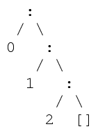
A non-empty list has a construction of the form x:xs, where : (pronounced cons) is an infix constructor. x is the first item (the head) of the list, and xs is the list of remaining items (the tail). Convention dictates that lists have an s suffix to denote that it is plural.
The type [t] includes lists of all lengths. [] is a list 0 items, and if xs:[t] is a list of n items, then for any x::t, (x:xs)::[t] is a list of n + 1 items.
By convention, : is right associative, so the list 0 : 1 : 2 : [] :: [Int] consists of 3 items, and the constructions looks like so:
Some useful abbreviations are also available, using the [ ] construction syntax. The above list, for example, could be constructed using [0,1,2], or alternatively to construct lists of numbers, using [0..2].
String is a synonym for type [Char], and strings can be represented as "hello", which is identical to ['h','e','l','l','o'].
User-defined Data Types
New data types are defined by type equations. The LHS of a type equation is often just a type name, and the RHS specifies alternative forms of construction by giving constructor name and components types, with each alternate form separated by a vertical bar.
data Primary = Blue | Red | Yellow
data Road = M Int | A Int | B Int | Local Name
data Accom = Hotel Name Size Standard | BandB Price
Type synonyms can also be defined, e.g., type Name = String or type Price = (Int,Int).
You should note that = here does not mean assignment, rather definition.
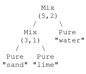
It is also possible to have recursively defined types, e.g., data Substance = Pure String | Mix (Int,Int) Substance Substance. A value representing mortar may therefore be Mix (5,2) (Mix (3,1) (Pure "sand") (Pure "lime")) (Pure "water"). A diagram of this construction would look like:
Functions
A function is a rule determining a unique result value, given an argument value.
For any types a, r, there is a type a->r whose values are functions with an argument type a and a result type r.
Functional types don't have constructors. Non-primitive functions can be defined by equations, or expressed as lamba expressions.
If f::a->r and x::a are expressions, then f x :: r is an expression meaning the result of applying function f to argument x.
Evaluation
Evaluation (sometimes called reduction) is the process of obtaining values for expressions.
We use the notation e ⇒ v to mean expression e has the value v. We also use the symbol ⊥ to mean undefined value. These symbols are not part of Haskell programs, they are simply notations about programs.
Curried Functions and Multiple Arguments
By convention, the -> symbol is right associative, but function application is left-associative and function results may themselves be functions. We can exploit these three facts so that multiple-argument functions can conveniently be represented as a single-argument function with a functional result - a curried function.
For a function f whose uncurried version has two arguments, currying works like so:
f :: a->b->r x::a y::b
f x y :: r
f x yields a function of type b->r.
Arithmetic Primitives
The following list contains five of the arithmetic primitives defined in the prelude: (+),(-),(*),div,mod] :: [Int->Int->Int].
Arithmetic can also be expressed infix style: x + y means the same as (+) x y. Identifiers such as div and mod can also be used infix too, if back-quoted: 20 `div` 3 means the same as div 20 3. This backtick style can be used to make any operator infix.
One caveat to be aware of is that function application is like an invisible operator with the highest precedence. f x + y means (f x) + y, not f (x + y).
Constructor Functions and Polymorphism
The non-constant data constructors are functions for combining values.
For lists of Int items, such as 1:2:[], we need (:) :: Int -> [Int] -> Int, but for lists of Char items, such as 'a':'b':[], we need (:) :: Char -> [Char] -> [Char].
In fact, since list elements may be of any type, for all types t we will need: (:) :: t -> [t] -> [t].
This is a legitimate type, and we refer to t as a type variable. It is distinguished from constant type names by an initial non-capital. Types containing these type variables are polymorphic, and functions with these parametric polymorphism always do the same thing, whatever instance of their type is being used.
As well as the built in polymorphic types, we can also define our own polymorphic constructions, for example to define a polymorphic tree, we could use: data TreeOf a = Leaf a | Branch (TreeOf a) (TreeOf a), where these Leaf and Branch constructor functions have types: Leaf :: a -> TreeOf a and Branch :: TreeOf a -> TreeOf a -> TreeOf a.
Projectors
Projector functions are often defined to access the component values of constructions. e.g., non-empty lists have head and tail components, and pair types have first and second components.
Where there is more than one type of constructions, projectors are often partial functions, e.g., head [] = tail [] = ⊥.
Defining Values by Equations
To bind a value to a name, we make a definition comprising one or more equations. A preceeding type declaration optional. The simplest form of definition is a single equation with a name as the left hand side, and an expression as the right hand side.
linelength :: Int
linelength = 80
fullname :: String
fullname = title ++ forename ++ surname
The above example uses the list concatenation operator (++) :: [a] -> [a] -> [a], which is defined in the Haskell prelude. It is important to note that these are definitions of fact, and not assignments.
Functions
When a functional value is being defined, the left hand side can take the form of a curried application to one or more arguments. These left hand side arguments are patterns, built with variables, constructors and brackets. It is possible for there to be several equations, each catering for different argument patterns. The right hand side of each equation is an expression possibly involving variables from the left hand side.
When executing a function, the equation used is always the first whose left hand side patterns match the actual arguments, therefore this is one case where ordering is important. The language designers felt this was necessary to avoid ambiguity and overly verbose programs. e.g., p `implies` q can be expressed as:
implies True False = False
implies p q = True
by using the ordering trick, but if ordering was irrelevant, the only unambiguous way involves expressing the full truth table.
The expression for the result is derived from the right hand side by substituting corresponding argument components for pattern variables.
If no left hand side matches an application, then the result is ⊥
Sometimes, a definition may only have a single equation, but bind values to several names. In this kind of definition, the left hand side is a pattern whose variables are names being defined and the right hand side is an expression whose values match the left hand side pattern.
We can also use the _ symbol as an anonymous variable that indicates (a component of) a pattern that is not relevant to the equation in which it occurs.
Recursion
Every general purpose programming language provides functionality for the expression of recurrence in some form. Most procedural programming languages use loops, whereas functional languages use recursion as the basic tool, with control abstractions defined as required.
Generally, to ensure useful recursion and to avoid useless circularity, define at least one simple case (a simple case is an application that does not use recursion), and in each recursive application, the arguments should be simpler than the case being defined (i.e., close to a simple case). These rules are not hard and fast, and may be broken if you know what you are doing.
Functions with arguments that consist of a recursive data type t (e.g., a list) are often defined using a method called structural recursion, that is, with an equation for each different t constructor.
For constructions without any component of type t, the result is expressed simply, without recursion. For other constructions, the result is expressed recursively, that is, in terms of the results of applying the function to each component of type t.
e.g., for a list argument, we can make [] the simple case, and x:xs a recursive case, because of xs, so for a function length xs, then length [] will be an expression not involving length (in this case length [] = 0), and length (x:xs) will be an expression involving length xs.
Although the Int type is not recursively constructed, it is often convenient to define functions of the non-negative integers as if there were two forms of construction: 0 and n+1. For this reason, +1 is allowed in argument patterns where it plays the role of a quasi-constructor.
For functions of a non-negative integer argument, frequently we can now make 0 a simple case, and n+1 a recursive case.
For example, we could define replicate x n to yield a list of n x's:
replicate :: a -> Int -> [a]
replicate x 0 = []
replicate x (n+1) = x : replicate x n
Strictness
A function f is strict iff f ⊥ ⇒ ⊥.
It is strict if in its nth argument if f ... ⊥ ... ⇒ ⊥, no matter what the other argument values are.
Here, ⊥ is a value nothing is known about - type may be known, but construction and properties not. Therefore, we can say that strict is if nothing is known about the argument, then nothing is known about the result.
Some predefined strict functions include the character coding functions ord and char (to know the ASCII code, you need to know the character, and vice versa), the list projectors head and tail (e.g., head ⊥ ⇒ ⊥, because if nothing is known about a list's construction, then we don't even know if it has a first item, let alone what that item is), and the arithmetic functions (+), (-), (*), div and mod (we can say that the arithmetic functions are strict in both arguments - e.g., to know the value of m+n, we must know the values of both m and n).
Polymorphic Equality Test
Equality testing is defined for each type belonging to the Eq class: (==) :: Eq a => a -> a -> Bool.
All the types in the Haskell Prelude belong to Eq if their component types do. Functional types, however, do not belong to Eq, as function equality is undecidable (thanks to the halting problem).
It is important to not confuse == with =. == is used in expressions to test equality; = is used in equations to assert equality.
We can also say that (==) is strict in both its arguments; if we don't know about one of the arguments, we can't say whether it is the same as the other.
Constructors
Functional constructors are by default non-strict in all their arguments. e.g., one may still know about a (:)-constructed list, even if nothing is known about its tail. O:⊥ is not the same as ⊥ - head (0:⊥) ⇒ 0.
Even if nothing is known about the head of a list, a (:)-constructed list is not just undefined; ⊥:⊥ is not the same as ⊥.
Later, we find that non-strict constructors will be the key to computing over infinite data structures. We do not need to know about all the components to know something about the structure as a whole.
Pattern Equations
⊥ can be substituted for variables when matching arguments against patterns, however we cannot say whether ⊥ matches a construction, so any application involving such a match ⇒ ⊥.
Conditions
Logical conjunction and disjunction are predefined as functions strict in their first argument, but non-strict in their second argument.
(&&) :: Bool -> Bool -> Bool
False && y = False
True && y = y
(||) :: Bool -> Bool -> Bool
False || y = y
True || y = True
We can also consider a cond function defined by:
cond :: Bool -> a -> a -> a
cond True x y = x
cond False x y = y
This is strict in its first argument - we need the value of the condition to determine the correct branch, however it is non-strict in both other arguments - we do not need to know about one or other of the alternatives.
As an alternative to this cond function, there is a special but familiar notation for something equivalent: if c then x else y, which is equivalent to cond c x y. This "distributed-fix" notation has lower priority than function application or any infix operator.
Conditions can also be specified at the definition level, e.g., f n | n > 0 = ....
Local Definitions
Before now, all definitions were flobal, howeer, the right hand side of a defining equation may incorporate local definitions:
equation
where
local equations
Things in the parent scope (i.e., that of equation) are still in scope of the local definitions.
Local definitions make it easy to keep together a definition and all of its uses, enable defintions to be split into pieces of suitable size for a human reader, and eliminates the need for some function arguments, since local definitions may refer to variables on the left hand side of the main equation. Local definitions also avoid problems of naming conflicts that may arise in larger programs, and they provide a way to avoid repeated occurences of the same subexpressions - and perhaps repeated evaluations of it too.
Languages without local definitions may be smaller and simpler, but programs may need to defined more functions with more arguments.
Local defintions have come in and out of favour repeatedly over the years. Circa 1975, SASL had local definitions, but circa 1980 KRC had none in an experimental language. In 1985 they were re-introduced in Miranda, and then kept in 1990 with Haskell.
There is also an alternate syntax for local definitions:
let
defns
in
expr
Projections of Recursive Results
When a recursively defined function computes a data structure as its result, to refer to components of a recursive result, it is necessary to bind it to a local pattern, rather than to use explicity projecions.
Auxiliaries
For an example see
page 38 of the lecture slides.
An auxiliary function is a function which exists to help another function do it's job.
The choice of auxiliary functions often determines the simplicity of solutions, as many auxiliaries are intended to handle specialised sub-problems. Auxiliaries may also correspond to generalised super-problems, however. The main method used to generalise a function is to introduce auxiliary arguments.
Auxiliary arguments come with two conflicting intuitions. The first is that the additional arguments mean additioonal work, so definition is more complex, but the second is that addition arguments mean additional information, so the definition becomes simpler. Neither of these intuitions are are adequate alone, so the potential validity of both needs to be realised.
The most useful argument to be supplied to a function is the answer to the function. This is obviously not going to be the case for most functions, but an argument known as an accumulator can be used to carry a partial construction of the result to be computed. Recursive applications extend the construction of the accumulator value.
To formulate a basic structure-recursive definition of a function f over lists, we study the relationship of f xs and f ys to f (xs++ys).
A good rule of thumb is to introduce an auxiliary argument for each maximal subexpression of the right hand side involving xs, but not ys.
Higher Order Functions
A higher order function is one that takes an argument of functional type, or yields a result of functional type.
Curried functions are higher order since they represent multi-argument functions as single-argument functions with a functional result. Higher order functions can be used to provide parametrised recursion schemes, reducing the need for explicit recursion from scratch.
Polymorphic types are particularly valuable in the case of higher order functions.
map applies its first argument (a function) to each item of its second argument (a list) and yields the list of results. For example:
map head ["Value","Added","Tax"] ⇒ "VAT"
filter is another higher-order function for list-processing. Its first argument is a predicate p, and its second a list xs. Its result is a list of the items in xs that satisfy p, for example:
filter set ["every","one","a","winner"] ⇒ ["one","a"]
Generalised Lists
foldr expresses a more fundamental list-processing pattern. It computes generalised lists, that is, its result is a reconstruction of a list using a given function f in place of (:) and a given value z in place of [].
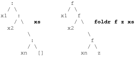
foldr's type reflects the asymmetric nature of lists: foldr :: (a->b->b) -> b - > [a] -> b.
foldr's defining equations make clear the list recusive pattern of computation that captures:
foldr f z [] = z
foldr f z (x:xs) = f x (foldr f z xs)
Intuition tells us that completely replacing all constructors is a very general way of recombining components, and we can observe that foldr can be used for a surprisingly wide variety of computations.
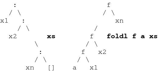
foldl is a mirror image of foldr. foldl captures the list-accumulation scheme, as its definition reveals:
foldl :: (a->b->a) -> a -> [b] -> a
foldl f a [] = a
foldl f a (x:xs) = foldl f (f a x) xs
Higher order functions can be obtained by auxiliary argument generalisations. e.g., if we define sum like so:
sum [] = 0
sum (x:xs) = x + sum xs
What makes this "summy" is the use of 0 and +. We can make sum more generally applicable by replacing 0 with an auxiliary argument z, and by replacing + by an auxiliary argument f, i.e.,
gensum f z [] = z
gensum f z (x:xs) = f x (gensum f z xs)
gensum is now just foldr by another name.
Partial Application
If f is a curried function of n arguments, it can be applied to fewer than n (say m) arguments. The result here is a function of n-m arguments, that is, a specialised version of f with the first m argument values "frozen in". e.g.,
contains :: Eq a => [a] -> a -> Bool
contains [] e = False
contains (x:xs) e = x==e || contains xs e
punctuation :: Char -> Bool
punctuation = contains ",;:.!?"
Such a partial application complements the technique of auxiliary argument generalisation. It enables us to make fuller use of higher order functions that necessarily assume functional arguments of a particular arity.
Parital applications of binary operators benefit from a special notation: e.g., (5-) or (:[]), and are sometimes called operator sections.
Function composition is to functional programs what statement sequencing is to procedural programs: (.) :: (b->c) -> (a->b) -> (a->c), so (f . g) x = f (g x). This ability to compose functional arguments using (.) further enhances opportunities to use higher order functions.
The (.) operator is a function level primitive - all its arguments and its results are functions. Many defining equations for functions can be cast entirely at a functional level too: arguments of data type need not be mentioned.
For example, if we had a function inter xs ys = filter (contains xs) ys, both the left hand side and the right hand side apply a function to ys. By definition, for every argument ys, their results are the same, that is, they are the same function. It is therefore equivalent to define: inter xs = filter (contains xs). Now, the RHS is a composed application, that is: inter xs = (filter . contains) xs. And just as we eliminated ys before, we can now eliminate xs: inter = filter . contains.
Although the arguments may be unmentioned in a function-level definition, they are still implicit in the types of the functions.
Redexs and Normal Forms
A reducible expression (called a redex) is an instance of the left-hand side of a defining equation, but not an instance of any earlier equation, or a primitive application to which a primitive rule of computation immediately applies.
A normal form is an expression containing no redex.
e.g., both 2+3 and contains [] 0 are redexs, and the normal forms to which they reduce are 5 and False respectively.
These expressions are not redexs, though they contain two redexes as subexpressions: (3-1) + (5-2) and contains (tail[6]) (head[0]).
Running a functional program on a single-processor computer requires some evaluation strategy to select and reduce successive redexes until a normal form is reached.
Fortunately, normal forms are unique - different strategies applied to the same expression can not lead to different normal forms.
However, some strategies are less efficient than others, requiring more reductions to reach normal form starting from the same expression. Some strategies, though efficient for many expressions, are infinitely inefficient for others. They may fail to terminate, even though there is a normal form that could be reached in a finite number of steps.
Here, we refer to efficiency as the number of reductions, but it is important to bear in mind that the housekeeping may be complex.
Eager Evaluation
To evaluate a function application, the eager strategy of applicative order, or innermost reduction, first evaluates the argument to normal form. Semantically, the effect is to make all functions strict. A similar call-by-value rule is usually assumed for procedure calls of imperative languages.
Lazy Evaluation
The lazy strategy of normal order evaluation always reduces the outermost redex available. Semantically, this makes non-strict functions possible. A similar call-by-name rule is available in some imperative languages, but it is little used.
Under this strategy, arguments are evaluated zero or more times, as often as they are needed. The strategy always reaches a normal form if one exists.
This form of evaluation is considered to be näive. We can be lazy efficiently by using normal order graph reduction. This avoids repeated evaluation of arguments by representing expressions as graphs rather than as trees. All uses of an argument then point to a single shared representation of it, so that when it is reduced, all uses feel the benefit.
Pattern Driven Reduction
Several outermost redexes may be subexpressions of an enclosing (non-redex) function application. If the enclosing application is a constructor, its components are evaluated left-to-right, otherwise the enclosing application must lack the information needed to match an equation left hand side - the matching strategy is top-to-bottom and left-to-right.
Infinite Data Structures
Functional valures comprising infinitely many argument-result rules can be defined recursively. It therefore follows that data values with infinitely many components can also be defined recursively, e.g.,:
white :: String
white = ' ' : white
nats :: [Int]
nats = 0 : map (+1) nats
The second form of an infinite data structure can be represented more concisely as nats = [0..].
Many data structures are naturally infinite. We can only use a finite part of them in any one computation, but that does not need to force us to set limits specifying which part.
Although this data structure has a finite representation, it is infinite and from the users point of view is the same as an infinite foldr with a spine of :.
Lazy evaluation provides a means of computing exactly those parts of an infinite data structure that are needed for a particular computation. For example, with the nats example:
The last element in the list has not been used yet, and is waiting to be unrolled.
Lazy Tabulation
To tabulate a function, we can list its results for all arguments in order. Assuming natural number arguments, we can define:
table f :: (Int->a) -> [a]
table f = map f [0..]
Looking up a result in such a table is a linear operation, defined like so:
(x:_) !!0 = x
(_:xs) !!(n+1) = xs!!n
Using table and (!!) we can arrange for amortised linear computation of any function of the naturals without abandoning the structure of a specification-based definition.
Set Comprehensions
In some ways, lists are like sets. They are collections of elements, but ordered, and may contain repeats. In Maths, sets are often defined by comprehensions such as : S = { n2 | 1 ≤ n ≤ 10, odd(n) }.
In that example, the boolean conditions are all we have to constrain or generate appropriate elements n. But the condition can often be expressed as an extra requirement on elements drawn from a known set, e.g., S = { n2 | n ← {1, ..., 10{, odd(n) }. This is a relative abstraction.
This kind of comprehension is available for lists in Haskell. The above example expressed in Haskell would be s = [n*n | n <- [1..10], odd n].
The qualifiers <- are generators that bind successive items from a given list to fresh variables. These variables are in scope to the right of the qualifier and in the expression to the left of the |. The other qualifiers are constraints expressed as boolean expressions, they do not introduce fresh variables. This is called the generate and test paradigm.
More generally, the syntactic forms of a comprehension for a list of type [t] include:
comp = [ t-expr | qual_1, ..., qual_n ]
qual = var <- list-expr | bool-expr
We could define the meaning of comprehensions directly, using extra rules of evaluation. But they can also be translated into other forms of expression like these:
[e | c] => if x then [e] else []
[e | quals-prefix, quals-suffix] => concat [ [ e | quals-suffix] | quals-prefix ]
[ e | v <- list ] => map (\v -> e) list
Implementations do something equivalent to these translation rules, but can often be more efficient. For example, the comprehension [ x | x <- xs, p x ], is intuitively equivalent to just filter p xs, but the translation rules give us something a lot more verbose.
If a comprehension has more than one list generator, all combinations of elements (that satisfy any boolean qualifiers) are generated. Rightward generators iterate within leftward ones, e.g.,
[(x,y) | x <- [1..3], y <- "ABC"]
==> [(1,'A'), (1,'B'), (1,'C'), (2,'A'), ..., (3,'C')]
This is at the expense of a slightly more complex translation rule, instead of just a simple variable on the left of <-, there may be a pattern with the effect that only elements matching the pattern are drawn from the generating list.
Sometimes we don't want all combinations of elements from two lists, but only a combination of elements at corresponding positions. The function zip :: [a] -> [b] -> [(a,b)] is handy, e.g., positions xs x = [n | (n,y) <- zip [0..] xs, x==y].
An apparently distinctive feature of logic programming is its support for multiple results, reached by back-tracking to find alternatives. We can do the same thing in a lazy functional language, just using lists of alternative results. Even if there are ininitely many alternatives, they are only computed if they are needed.
Interaction
Processing Message Streams
Functions computing over infinite lists can also be viewed as processes communicating with their context by streams of messages. Argument items correspond to messages received, and result items correspond to messages sent.
Programs can be constructed as networks of such processes operating (conceptually) in parallel.
These networks can often be expressed diagrammatically, using circles representing functions, and a triangle representing :. Solid lines represent potentially infinite lists of items, and dashed lines indicate a single item.
Until now, program execution has involved the user supplying one input - an expression. This is reduced to a normal form, and then printed.
If results are values, then what about interactive behaviour?
We can formulate programs that take input beyond an original expressiong by defining a function f :: String -> String, and then arrange to supply the list of characters entered at the keyboard as f's argument, and for its result to be the list of characters sent to the screen.
Unless f is hyper-strict or tail-strict (that is, it must know everything about its arguments before returning), such a program described above behaves interactively. The lazy reduction strategy ensures that its output is suspended only when a further portion of input is strictly needed.
Monads are another way to implement interactivity, and are fashionable at the moment, but are not being covered by this course.
Page 71 of the lecture notes
It is often convenient to define two line-based auxiliaries to provide line-based, rather than character-based, interaction. lines chops text into lists of lines, and unlines assembles lists of lines into text. The first can be defined by a recursive application of breakAt and the second is easily defined as a composition of concat and map, but a foldr version is more efficient.
A simple scheme for line-based interaction is the simple command-response loop, in which the same function is applied to each command (line of input) to yield a response (line of output).
If we require prompts, then the solution is slightly more complicated. One way is to merge a stream of prompts into the output, using the repeat function and the interleave auxiliary, defined as:
interleave [] _ = []
interleave (x:xs) ys = x : interlease ys xs
Stately Mappings
Using map means that the same function is applied to interpret every command. No information from an interaction is carried forward for later use. One way to overcome this is to generalise map, introducing state as an auxiliary argument.
By using this new mapState in the place of map, our scheme for expressing interaction can be enriched further.
It is often useful to think of these as message streams at a process level, e.g.,
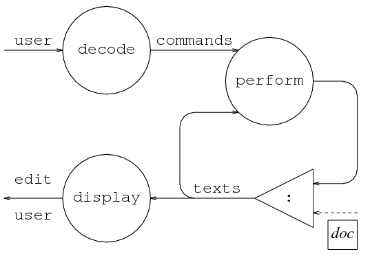
We also need to consider what type each of the message streams between processes should have. In our previous example, the type of user is already determined by interact as a String - the list of characters entered at the keyboard.
We can represent distinct commands as distinct constructors: data Command = Ins Int String | Del Int, and assign the type [Command] to this stream.
Lines can sensibly be given a type string, so a simple text representation is a list of lines, type Text = [String], giving [Text] as the type of the texts stream.
As the result of edit is a list of characters sent to the screen, edit user must also be a String.
In the above process diagram, we should also consider the individual processes. For the decode process, each line from user is interpreted similarly using the bufferedLines and map auxiliaries. Each line must be then split into either two or three fields, depending on the command, using the breakAt ' ' auxiliary, and we also need to convert numerals into integers where appropriate using the strint auxiliary.
For the perform process, each combination of a command and a text is interpreted by the same rules, using the zipWith function. Intuition tells us that we can fulfull each command by cutting the text in two at the specified line number, inserting or deleting text at the cut and rejoining the text. The auxiliaries take and drop can be used to cut, and then ++ can be used to rejoin.
To express the display resulting from an entire session for the display process, we can just concat the successive text displays. As each text is displayed in the same way, we can just use map, and zipWith to attach line numbers.
As you can see, this problem was factorised by beginning with a process level design, and explicit recursion in the definitions of processes was avoided by using higher order functions. The remaining definition work was minimised by using polymorphic auxiliaries. No conditionals were needed, because all case analysis was done by pattern matching.
More intrusive extensions and comparisons can be considered, such as a more efficient representation of text supporting the introduction of a current line-number, or an undo command (although) it is surprisingly easy to modify the perform process to receive and send text histories, say as lists of texts.
Transformation
A common problem is that a function may have many different possible definitions. Definition A may be simple and obviously correct, but inefficient in computation, but a defintion B may be far more efficient, but also more complex or subtle.
The transformational approach begins by formulating a simple definition, ignoring efficiency concerns, and then applying transformational rules to derive new equations guaranteed to define the same function, but chosen to do so more efficiently.
- Eureka - the inventive formulation (e.g., fstCol ys = map head ys)
- Instantiate - substitute a constructor pattern for a variable in an existing equation (e.g., instantiating ys to [] and (x:xs)).
fstCol [] = map head []
fstCol (x:xs) = map head (x:xs) - Unfold - apply one defining equation in another, replacing a left hand side instance by corresponding right hand side (e.g., unfolding map in each of the above equations)
fstCol [] = []
fstCol (x:xs) = head x : map head xs - Fold - the inverse of unfold (e.g., appealing to the original fstCol equation)
fstCol [] = []
fstCol (x:xs) = head x : fstCol xs - Abstract - introduce a local definition (e.g., if we already have the equation fib (n+3) = fib (n+1) + fib n + fib (n+1) we may derive:
fib (n+3) = f + fib n + f
where
f = fib (n+1) - Law - substitute for one expression another known to be equivalent by appealing to axioms about primitives, or theorems about explicitly defined functions. (e.g., another reformulation of the fib equation achieves a similar economy by a law of arithmetic: fib (n+3) = fib n + 2 * fib (n+1)
This system of six equation-forming rules is known as the fold/unfold transformation system. It should be noted that folding and unfolding here does not refer to foldl and foldr.
A good general strategy to follow is: eureka (make some definitions); instantiate equations of interest; in each instantiated equation, unfold repeatedly and try to apply new laws, abstract local definitions and fold in new places.
Some commonly applied heuristics for new definitions include:
- composition/fusion - if some composite application f .. (g .. ) .. has g producing a structure that f dismantles, make this composition a defined function in its own right. Transformational composition replaces an indirect route from an argument to a result by a more direct route, e.g., avoiding building intermediate lists.
- generalisation - if folding proves difficult because some subexpression of the relevant right hand side does not match, generalise the original equation so that the right hand side has an auxiliary argument variable at that point.
- tupling - if two or more subexpressions involve recursive computations over the same argument, say f .. x .. and g .. x .., introduce a function that computes the tuple of these results. Intuition tells us that tupling replaces independent travel of a common argument by shared travel as far as possible
Often, one (cheap) auxiliary function is applied to the result of another (recursive and comparatively expensive) auxiliary, to obtain a desired result, e.g.,
prog xs = extract (fun xs)
fun [] = c
fun (x:xs) = f x (fun xs)
Suppose we want a directly recursive defintition of a function, the usual fold/unfold strategy would give us the equation:
prog (x:xs) = extract (f x (fun xs))
But the intervening f x prevents a fold. If extact and f x could change places, then we could fold. The promotion tactic is to calculate an f′ such that extract . f x = f′ x . extract, hence creating the desired opportunity for a fold: prog (x:xs) = f′ x (extract (fun xs))
Retaining Strictness
If we consider the reduction of a function application by appeal to the defining equations of the function, then:
- if an argument is never matched against anything more than a simple variable, the function may or may not be strict in that argument;
- if an argument is matched against a constructor pattern, the defined function is strict in that argument;
- instantiation replaces simple variables by constructor patterns;
Therefore, an instantiated definition will be strict, whether or not the original was. This means that a change in meaning due to instantiation in a non-strict context can be quite subtle, but its effects are all too apparent when the function is used interactively. For complete inputs, examining only the complete result printed, given a complete input sequence may result in no apparent problem, but for partial input problems become apparent.
Adding instances creates an implicit equation f ⊥ = ⊥, so you mean consider the situations of f ⊥ and f (x:⊥).
To achieve safe instantiation, we must check before instantiate whether the function is strict in the instantiated variable, as only strict instantiation is safe.
To handle non-strict functions, instead of instantiating the definition of the entire non-strict function, we apply a similar instantiation to a maximal strict auxiliary. One intuition tells us do this by peeling away the thinnest possibly layer of non-strict material to reveal one or more strict functions underneath, but another intuition tells us to extract the largest possible strict expressions surrounding the actual uses of the variables to be instantiated.
To extract safe auxiliaries, we first unfold as far as possible without instantiation, and then subsitute ⊥ for the argument and unfold ⊥ results only. Compare the before and after results and define a strict auxiliary, folding it back in to the before result.
Proving Equivalence
How can we establish whether two functional expressions are equivalent? (i.e., interchangable). Testing for equal results across a range of arguments is of limited use (there may be an infinite number of possible arguments, and when one or both results is ⊥, the result of == is itself ⊥, not True as required). Indeed, automatic checking is not feasible by any algorithm, because the equivalence problem is undecidable.
Proof of equivalence as a law or theorem appears to be necessary. We can expect inductive proofs because we have recursive definitions. Fold/unfold can be regarded as a kind of proof, though we have not been rigorous about the inductive assumptions involved.
Natural Induction
Using natural induction, to show a proposition P n holds for every natural number n, it suffices to show P 0 and assuming P n holds, P (n+1) follows.
If n ranges over programmed expressions, whose results, if any, are natural numbers, we must also show: P ⊥.
Structural Induction
To show a proposition P v holds for every fully-defined value v of some data type t, it suffices to show:
- for every constant constructor C of type t, P C holds;
- for every functional constructor F of type t, if ∀i . P vi holds, where i ranges overs positions of F's arguments of type t, then P (F v1 ... vn) follows.
To extend this to cover (partially) undefined values of type t, we must also show P ⊥.
Applying this scheme to a list type, for example, P is true of every type-compatible list expression if:
- P [];
- if P xs holds, P (x:xs) follows;
- P ⊥