Computer Science notes ⇒ COM6460: Speech Technology

Classification is the task of assigning a sample to a particular class in a finite set (e.g., a phoneme, word or speaker), hence most speech technology tasks use classification techniques. The most complex speech technology task is automated speech recognition (ASR), but most other tasks derive their algorithms from ASR principles.

Pattern classification is one of the most important tasks in pattern processing. The task is to identify patterns in the input data such that the data can be assigned to one out of a finite number of classes C_i. All pattern processing techniqes make use of the fundamental pattern classification paradigm: Given an example x, feature extraction is used to obtain a representative vector y, which can be classified into a class c.

The recogniser capabilities can be defined along a number of dimensions: speech, environment, linguistic criteria, input/output forms, internal specifications and the recogniser platforms. For types of speech, classifications include the mode of speaking (e.g., isolated word, short phrases or continuous speech), the speaker set (single speaker (can be trained to be dependent), multi-speaker or any-speaker (must be speaker independent)). Most speaker independent systems make assumptions about accent subsets and a modern trend is towards speaker adaptive systems.

When considering environmental factors, noise is a key factor (whether the environment is noise-free, in an office or high-nouse) and whether this noise condition is fixed or adaptive. An additional factor is that of the microphone or channel (e.g., close-talking, far-field, telephone, etc).

Linguistic criteria can also be considered for classification of ASRs: their vocabulary (very small ≤ 20 words, small ≤ 200 words, medium ≤ 2000 words, large ≤64k words or very large > 64k words), their syntax (non-existant, finite-state, context-free - possibly stochastic - or n-gram) and the language domain (single language, multi-language, etc) they work in. Some ASRs also support multi-modal input, such as combined modelling of lip-reading, gesture or speaker identification.

Other classifications include that of system output, whether it gives multiple hypotheses (possibly ranked) or possible outputs, confidence scores for each word in the output or "rich transcripts", which are human readable. The internal representation of the system can also be considered - whether it stores representations of words or sub-words (phones), which are more flexible and allow for vocabulary independence.

Low error rate is one common metric used. This compares the output of the output string with a manually transcribed version (reference transcript) and the word error rate is the percentage of words that were different.

Another common metric is user satisifaction. As recognisers form part of a larger system, users are more interested in the overall system performance rather than the raw error rate.

It is necessary to integrate the recogniser (and its shortcomings) into the design of a system so that it can cope with recognition errors (e.g., by using confirmatory dialogue and allowing correction).ASRs historically have worse performance in the field than the lab, hence the collection of realistic databases for development and test is necessary.

In ASR, our task can be reduced to finding the most likely sentence (word sequence) W used for generating the utterance A: W^ = max_WP(W|A). By Bayes rule, we can rearrange this to W^ = argmax_WP(A|W)P(W). In this model, we can consider P(A|W) to be the acoustic model and P(W) the langauge model. The ASR problem is then reduced to finding solutions for two problems: training (finding suitable representations for the acoustic model and the language model) and recognition (finding the most likely word sequence W^). The most common form for the acoustic model is a hidden Markov model (HMM), and for the language model, N-grams.

A generic ASR architecture typically consists of a speech processing front-end (providing A) and a vocabulary (providing W) along with the acoustic model (P(A|W)) and the language model (P(W)) all feeding into the search (argmax) which outputs the most likely word sequence. Often some feedback is introduced which alloes for adaptation of the langauge and acoustic models.

The front-end converts the audio into a stream of feature (observation) vectors. The acoustic model is responsible for matching acoustics and individual words as defined in the vocabulary and is the most complex part of an ASR system. The language model represents syntactic, semantic and discourse constraints on the output string (ensuring what is output is valid), and in some cases no (or a null) model is appropriate. Words not in the vocabulary can cause errors.

Isolated word recognition simplifies the system by pre-segmentation of the speech data, however this is not straightforward in anything but a low-noise audio environment.

By far the most common front-end is based on Mel-frequency Cepstral Co-efficients (MFCCs). Typically overlapping (one every 10 ms) speech frames of 25 ms length are used. This is done to capture changes of speech over time and 25 ms is a good number to capture the quasi-stationary property of speech - phones are typically between 50 and 200 ms in length, although more often towards the shorter end of this range. Overlapping is done to avoid discontinuities.

A Hamming window is applied to stop spectrum distortion in the FFT phase. FFTs assume that signals are periodic, and not applying a window can lead to sharp edges ("leakages") in the signal. A Mel filterbank is applied and then log conversion of the signal and a discrete cosine transform applied to arrive at a feature vector of the MFCCs. Normally the 0th cepstral coefficient is excluded, so a measure of raw energy needs to be added to the feature vector.

Mel-scale filterbanks use band analysis to model masking effects by the ear together with non-linear frequency and bandwidth allocation. The energy in each frequency band can be computed by DFT. Phase information can be disgarded as experimental results show that humans can not differentiate between identical sinusoids with different phases. The spacing of the centre frequencies is based on the Mel-scale, defined as: Mel(f) = 2595 log₁₀(1 + f/700). This is often regarded as being approximately linear up to 1 kHz and then logarithmic thereafter.

Cepstral coefficients can be derived from the Mel filterbank energies using a simplified version of the DFT known as the discrete cosine transform (DCT), which takes advantage of the fact that the log magnitude spectrum is real-valued, symmetric with respect to 0 and periodic in frequency:

c_n = √2/P ∑^P_i=1m_icos((n(i - 1/2)π)/P), where P is the number of filterbank channels.

The DCT decorrelates the spectral coefficients and allows them to be modelled with diagonal Guassian distributions. The number of parameters needed to represent a frame of speech is reduced, in turn reducing memory and computation requirements. c₀ is a measure of signal energy.

MFCCs describe the instantaneous speech signal spectrum, but take no account of signal dynamics. Moreover, the use of HMMs requires that dynamic information is packed into local vectors because of the assumption of frame independence. This situation can be improved by including rates of change of the coefficients (differentials) in the representation. Typically, regression coefficients are used to calculate the best straight line through a number of frames:

R_n(t) = (∑^δ_τ=-δτc_n(t + τ)) / (∑^δ_τ=-δτ²)

For similar reasons, the representation can also be augmented to include the second differential of the static coefficients by again applying the regression formula to the first order differentials. For HMM-based speech recognisers, a modern standard representation includes static, Δ and ΔΔ coefficients.

Any fixed linear filter that is applied to the speech (such as a microphone) causes the measured speech spectrum Y(ω) to be the product of the original speech S(ω) and the frequency response of that particular filter H(ω): Y(ω) = S(ω)H(ω).

Taking the logarithm (which can only be done on a magnitude spectrum) allows us to express this as: log Y(ω) = log S(ω) + log H(ω), and log |Y(ω)| = log |S(ω)| + log |H(ω)|, which shows that the distortion of the speech signal is additive.

If log |H(ω)| can be estimated, it can be subtracted and the measured speech is then independent of the channel. This is derived from the idea that, within an additive constant, log |H(ω)| is the average value of log |Y(ω)| over the utterance (or set of utterances on the same channel), since it is assumed that on average log |S(ω)| is flat.

If y_t represents a frame of observed speech in the spectral domain, hence s_t + h_t, where h_t is assumed to be constant over time, then:

1/T ∑^T_t=1y_t
= 1/T ∑^T_t=1(s_t + h_t)
= 1/T ∑^T_t=1(s_t + h)
= Th/T ∑^T_t=1s_t
= h

Since the cepstrum is a linear transformation of the log spectrum, as are MFCCs. For MFCCs, the average cepstrum (e.g., over an utterance) can be subtracted from all the static coefficients. This is termed cepstral mean normalisation (or subtraction or removal).

Distance metrics are used to compare a speech vector o with another speech vector v. A distance measure d(o, v) is defined such that it is large if o and v are different, and small is they are similar.

Euclidean

Mahalanobis

For cepstral representations, any of the above distance measures are appropriate (since their distributions are close to Gaussian), however for LPC predictor coefficients, the Euclidean distance is not appropriate and often the Itakura distance is used.

Itakura

There are a number of instances where it is required to represent a continuously valued multi-dimensional vector by a discrete symbol. This process is called vector quantisation (VQ). This speech vector o is mapped to a scalar: o → k. A codebook C is then built up as a set of K centroid vectors (codewords, or representative values). The observation vectors are then mapped to a codebook symbol using k = argmin_1≤l≤Kd(o, v_t).

The set of codewords together with a distance metric provide partitioning of the space.

Linde-Buzo-Gray (LBG) algorithm

Centroid Splitting

For classification, the distance to the nearest codebook values are summed up and the classification with the smallest distance is used.

The Gaussian distribution is one of the most important probability distributions: P(x) = 1/σ√2πσ² e^{-(x - μ)2/2σ2}, where σ² is the variance and μ is the mean.

To give a score, two Gaussian models are learnt - one for male and one for female. The probabilities of P(O|male) and P(O|female) are then compared, where P(O|male) = ∏_tP(o_t|M), and similar for female, where these probabilities are drawn from the Gaussian distribution.

To learn these example parameters, then μ = 1/T ∑_to_t and σ = 1/T ∑_t(o_t - &mu)².

A simple detection approach to classify utterances is to compute the average distance of all feature vectors in the observation to a reference vector v_j for a particular word w_j. The word w_k with the minimal average distance is then selected. If we extend the concept to use a reference template of length T instead of a reference vector, then if the length is identical, to the observation we can compare the vectors one by one.

However, the length of the template is fixed and the length of the observation sequence varies, causing an alignment problem. When varying the length of speech, it is only some phones that change in length, not all phones linearly, therefore linear warping is inappropriate here, and non-linear warping is needed.

Dynamic time warping is a technique such that the total difference between two sets of vectors is minimal, and it can be implemented efficiently by the use of dynamic programming.

A Markov chain is a stochastic process based on state machines that can generate a random sequence that is discrete in time and value. The output of the process is a sequence of length T given by X = [x(1), x(2), ..., x(T)], such that the values x(t) are taken from some finite alphabet S = {s₁, s₂, ..., s_M}, representing the states the Markov model moves through.

Using Bayes, the probability of the output sequence can be computed: P(X) = P(x(1))∏^T_t=1P(x(t)|x(1), ..., x(t - 1)). A first-order Markov chain makes use of the independence assumption that the probability of a particular symbol at a particular time, x(t) only depends on the immediately previous symbol, x(t-1) - the Markov assumption. Hence, P(x(t)|x(1), ..., x(t - 1)) = P(x(t)|x(t - 1)).

In a first-order Markov chain, the probability of a sequence X is defined by P(X) = P(x(1))∏^T_t=1P(x(t)|x(t - 1)), where P(x(1)) is the initial probability of the sequence and the other probabilities are transition probabilities.

The set of initial probabilities is defined as: ∀1≤i≤M π_i = P(s_i), such that ∑^M_i=1P(s_i) = 1, i.e., the sum-to-one condition. We can have a single initial state by simply setting this π_initial = 1.0.

The transition probabilities are defined as: ∀1≤i≤M, 1≤j≤M a_i,j = P(x_t = s_i|x_t-1 = s_j), such that ∑^M_i=1P(s_i|s_j), 1≤j≤M, i.e., the probabilities of leaving a node must sum-to-one.

The sets of initial probabilities and transitional probabilities complete define the Markov chain. These parameters are constant (not a function of time) and therefore this process is stationary.

The alphabet defines the states, and the random sequence is generated by moving from one state to another state, with the state selections governed by the transition probabilities.

To learn the probabilities of a Markov chain, this is straight forward. To discover the initial probabilities, we look at the training sequences and then look at the frequencies of a state starting a sequence over the total number of examples. For transition probabilities, transition pairs in sequences are considered and the probabilities computed such that a_i,j = N(i→j)/N(j), that is, the frequency of that particular transition divided by the frequency of i.

In the case of Markov chains, the state sequence is identical to the observation sequence - each state produces a symbol which is uniquely associated with that state. Hidden Markov models can be viewed as an extension to Markov chains where the output o_t of a state j at time t is governed by some probability distribution called the output distribution.

A Markov model is "hidden" as the state sequence is hidden by not being directly mapped to the data, but instead mapped by the output distribution.

b_j(o_t) = P(o_t|x(t) = j), is used to represent this output distribution. The output distributions can be discrete, which usually requires quantisation of the feature stream O by the use of a vector quantiser. This observation data is filtered through a codebook k_t = Q(o_t), and b_j(o_t) = P(k_t|x(t) = j).

Output distributions can also be continuous, and is typically represented by a Gaussian, and the probability replaced by a probability distribution function. Other distributions can indlude Laplacians, mixtures of Gaussians, etc.

For speech, as HMMs output some state alphabet, not spectrogram vectors, output distributions are needed. We could associate states with codebooks, but there is no guarantee that always the same vector is used (so it is not discrete). Gaussian distributions are used instead. Speech signals consist of quasi-stationary segments of finite length can be reasonably well described by concatenation of small sound units (phones). Left-to-right HMMs can be used to model these properties. In a left-to-right HMM, each state can produce an infinite number of output symbols, before moving on to the next one (and no moving back, hence left-to-right). The initial and final state of the HMM is non-emitting.

HMMs generate random, stationary sequences. The procedure to generate a random sequence is:

1. Select an initial state according to the initial probabilities;
2. If the current state is emitting, generate an output symbol according to the output distribution of the current state;
3. Select the next state according to the transition probabilities from the current state, then move to the next state;
4. If the current state is emitting and has transititons other than to itself, repeat step 2.

If words are spoken in isolation, we can reduce the complexity of the search for the best word sequence. We assume that words are separated from each other (in a sentence) by detectable pauses. The task for the acoustic model is simplified to providing an estimation of probabilities for words individually.

The front-end produces a stream of feature (or observation) vectors: O = [o₁, ..., o_t, ..., o_T]. In continuous ASR, we have to search for the best word sequence W^ = argmax_WP(O|W)P(W), however if the audio stream can be separated by segmentation of the audio signal (so called end point detection) into M segments Oⁱ where i = 1..M, the sentence length (number of words) is directly derived from the audio signal.

Each audio stream Oⁱ is associated with one particular word out of a sequence W = [w₁, w₂, ..., w_i, ..., w_M] where the acoustic realisation of one word can be assumed to be independent of the neighbouring words. Thus, we can simplify the formula for continuous ASR to: W^ = argmax_WP(W)∏^M_i=1P(Oⁱ|w_i).

If words are assumed to be completely independent, we speak of word classification. Using a vocabulary of size N, we can choose the index of the likely word k = argmax_1≤i≤NP(O|w_i)P(w_i), where each word is really a hidden Markov model. This allows a linear search for the best matching model. If all words are equally likely (i.e., P is a uniform distribution), then we pick the word w with the highest likelihood P(O|w).

Using Gaussian PDFs for the output distribution, we can define an HMM by the transition probabilities a_i,j, which implicitly define the topology of the HMM, the mean vectors μ_i and the covariance matrices Σ_i, although typically only the diagonal covariance matrices are used (resulting in uncorrelated vector elements). These form a multi-variate Gaussian distribution.

If we can compute the likelihood of an observation sequence, we can use the earlier equation to select the most likely word. Models for each word in the vocabulary are needed, and this model is represented by the model parameters λ_w = {{a_i,j}, μ_i, Σ_i}, and the N word models make up the parameter set of the acoustic model: λ = {λ_w1, λ_w2, ..., λ_wN}.

The use of HMMs for ASR raises a number of questions: how to compute the probability of a given observation sequence O and a certain word w - P(O|λ_w), which is required for comparing word hypotheses in classification; what the most likely sequence that produced a given observation sequence is, knowledge of which allows timing information to be assigned to the audio stream which can be used for segmentation of speech data, as a simplified training scheme for HMM (as knowing a mapping of vectors to states makes this very easy) and for decoding; and how are the model parameters are chosen.

For choosing the model parameters, the parameters which achieve maximum likelihood over some training data is achieved (maximum likelihood estimation - MLE).

If the HMM parameter λ_w, the state sequence (or path) X and the observation sequence O are known, the likelihood for the joint event can be expressed in terms of output probabilities and transitions: P(O, X|λ_w) = P(O|X,λ_w)P(X|λ_w).

The probability of the state sequence is similar to Markov chains. Assuming that the initial (x(0)) and final (x(T + 1)) states are non-emitting: P(X|λ_w) = P(x(1)|x(0))∏^T_t=1P(x(t + 1)|x(t))

The likelihood of the observation sequence O given the state sequence is then: P(O|X,λ_w) = ∏^T_t=1P(o_t|o_t-1, ..., o₁, x(t)). However, as each observation is independent from the others, given the current state, then we can simplify this as: P(O|X,λ_w) = ∏^T_t=1P(o_t|x(t)).

The total likelihood of the feature vector stream O, given the model for a particular word λ_w = ∑_XP(O, X|λ_w), or using Bayes: ∑_XP(O|X,λ_w)P(X|λ_w), where ∑_X denotes the summation over all possible state sequences.

This definition of HMMs is based on independence assumptions: the Markov assumption (the probability of a transition into state j from state i is independent of previous states) and conditional independence (given a particular state at time t, the likelihood of the output symbol at that time is independent of any other state or previous output symbols).

However, these assumptions are problematic for the modelling of speech, since we expect smooth paramater trajectories, showing a strong correlation over time.

If both the state sequence and the observation sequences are known, a clear connection between any symbol in the vector stream and a state can be established. The feature vector stream also carries implicit informaation about time (e.g., one vector per 10ms). Ideally, all vectors associated with one state should belong to the quasi-stationary part of the speech signal, which allows the signal to be segmented in time. However, the state sequence is unknown (by the nature of a hidden Markov model), and one can not derive the original sequence with certainty, but given an HMM λ_w and an observation sequence O, the state sequence X* with the highest likelihood can be computed: X* = argmax_XP(O, X|λ_w), where the likelihood is given by:

P(O, X*|λ_w) = a_x*(0),x*(1)∏^T_t=1a_{x*(t),x*(t+1)}b_x*(t)(o_t).

a_x*(0),x*(1) is the initial probability, a_{x*(t),x*(t+1)} is the transition probability and b_x*(t)(o_t) is the output probability.

P(O, X*|λ_w) can serve as an approximation to the total likelihood. In this case, all other paths (competing state sequences) are assumed to provide only a minor contribution to the total likelihood.

The knowledge about the best state sequence allows us to temporally segment speech. This can be used to segment words into smaller units, sentences into whole words, or to enable a simplified training procedure of HMM parameters.

The trellis is another option to visualise the operation of an HMM. This provides us with a joint visualisation with the observation vectors over time, allowing us to plot the path through the HMM.

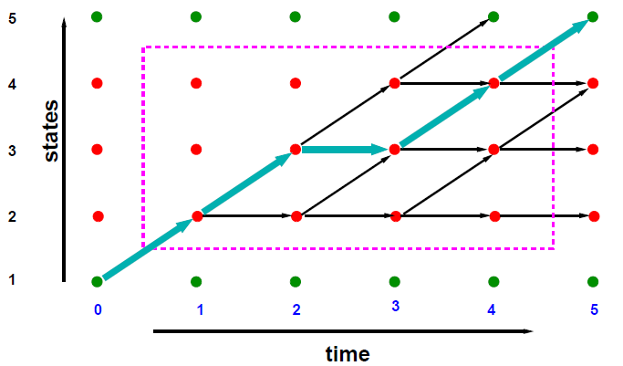
The most likely path through the trellis is depicted with the bold arrows, and the likelihood can be computed by the multiplication of the transitition probabilities (the arcs) with the output probabilities (the nodes). The non-bold arrows on the trellis indicate all allowed transitions.

The Viterbi algorithm is a dynamic programming procedure to obtain the most likely path for a given model λ and observation sequence O of length T.

First, we define the likelihood of a partial path of length t, which ends in state j: &Phi_j(t) = P(o₁, ..., o_t, x(1), ..., x(t - 1), j|λ)

Then, the likelihood of the partial path can be expressed in terms of the likelihood of the preceeding state x(t - 1): &Phi_j(t) = a_{x(t - 1),j}b_j(o_t)Φ_{x(t - 1)}(t - 1)

We can assume that our algorithm starts in the final state, as this state must be on the optimal path X*. We can now use the equation above to express the joint likelihood &Phi_N(T + 1) = P(O, X*|λ) in terms of the previous state: &Phi_N(T + 1) = a_x(T),N&Phi_x(T)(T).

Multiple paths may lead to the final state, however the optimal path is defined as the one which achieves the highest likelihood value P(O, X*|λ), thus one can select the preceeding state x*(T) such that &Phi_N(T + 1) is maximal: x*(T) = argmax_1≤j≤N(a_jN&Phi_j(T))

For simplicity, we use the notation k = x*(T). Once the state at time T is known, the partial likelihood Φ_k(T) can be expressed in terms of the predecessor state: Φ_k(T) = a_{x(T - 1),k}b_k(o_T)Φ_{x(T - 1)}(T - 1)

This includes the value for the output distribution at time T, so we again pick the preceding state that maximises Φ_k(t): x*(T - 1) = argmax_1≤j≤N(a_j,kb_k(o_T)Φ_{x(T - 1)}(T - 1))

This procedure can then be repeated for x*(T - 2), etc. In order to operate in this manner, the values for partial paths (Φ_j(t)) need to be precomputed. This leads to a forward pass, followed by a trace-back.

If we assume that an HMM M has N states, but the states 1 and N are the non-emitting entry and exit states, then the steps to obtain the most likely path X* and the associated likelihood are:

Φ₁(0) = 1.0
Φ_j(0) = 0.0 for 1≤j≤N
Φ₁(t) = 0.0 for 1≤t≤T
until P(O, X*|λ) = max_1≤k≤NΦ_k(T)a_kN:
    for t = 1..T:
        for j = 2..N-1:
            compute &Phi_j(t) = max_1≤k≤N(Φ_k(t - 1)a_kj)b_j(o_t)
            store the predecessor node pred_k(t)

The most likely path can then be recovered by tracing back using the predecessor information stored at each node in pred_k(t).

The Viterbi algorithm has the important property of being efficient, as decisions are local, paths merge and divide at roughly the same rate, and the time for the search is linear in the length of the observed data T.

One concern is that the direct calculation of likelihood will cause arithmetic underflow, this practical implementations of the algorithm uses the computation of log(P(O, X*|λ)): Φ_j(t) = max_1≤k<N[ log(Φ_k(t - 1)) + log(a_kj ] + log(b_j(o_t))

In this form, the search for the best state sequence appears as a generalisation of the template matching procedures used in dynamic time warping (DTW). DTW templates only represent a strict left-to-right topology, therefore in DTW the number of frames in the template is equal to the number of states, and all non-zero transition probabilities are equal.

In the case of a Markov chain, the knowledge about the state sequence allows us to compute maximum likelihood estimates for the transitition probabilities as discussed above, however for HMMs, the state sequence is unknown. Knowledge about the most likely state sequence X* allows us to approximate the total likelihood: P(O|λ) ≡ P(O, X*|λ). The knowledge of the state sequence X* clearly assigns each observation vector to exactly one emitting state.

Due to the conditional independence assumption, the parameters of each output distribution can be estimated independently using the data vectors assigned to a state. Formally, we can use an indicator variable δ to show if the observation vector at time t, o_t is associated with a state j: δ(x*(t) = j) = { 1 if x*(t) = j; 0 otherwise

See slide 20, handout 3
for the full formula.

This allows us to form an expression for the mean vectors and covariance matrices of the Gaussian output distribution for all states.

Another way of visualising δ is to consider the trellis as a matrix, with nodes on the most likely path given a value of 1, and others 0. Representing δ in this way allows for easy computation for the mean vectors and covariance matrices.

Viterbi training avoids the problem of hidden state sequences by use of the segmentation provided by the most likely state sequence, however the indicator variable δ represents a hard decision that the observation o_t is produced by the state j.

Baum-Welch re-estimation takes the uncertainty about the state sequence into account. The indicator variable is replaced by the state posterior probability: L_j(t) = P(x(t) = j|O, λ)

This can also be represented as a trellis, but instead of 1s and 0s, the number at a node represents the probability of being in that state j at time t in some Markov model λ given some observation sequence O. Total probability applies, so for a time t, the probabilities of being in a given state must sum to 1.

Any observation vector may occur with a certain probability at any time. The forward/backward algorithm is needed to provide an estimate for L_j(t). Similarly, the estimation of transition probabilities provides an estimate for P(x(t) = i, x(t + 1) = j|O,λ)

Forward algorithm

In order to compute L_j(t), it is necessary to define the backwards variable: β_j(t) = P(o_t+1, o_t+2, ..., o_T|x(t) = j, λ).

The definitions of the forward and abckward variables are not symmetric. Given both variables for a certain state j at time t: P(x(t)) = j, O|λ) = α_j(t)β_j(t).

See slide 27 of handout 3
for the full formulae

Using this information, an N-state HMM (with states 1 and N being non-emitting) and a Gaussian output distribution can be re-estimated using the update formulae. Multiple iterations of estimating the parameters are required.

The magnitude of α_i(t) decreases at each time step. This effect is dramatic in HMMs for ASR as the average values for b_i(t) are very small and leads to computational underflow. Two approaches have been used to solve this problem.

One approach is to scale α_j(t) at each time step so that ∑^N-1_j=1α_j(t) = 1. The product of the scale factors can then be used to calculate P(O|λ). Since this underflows, log P(O|λ) is found as the sum of the logs of the scale factors.

An alternative solution is to use a logarithmic representation of α_i(t). Many practical HMM systems use this solution.

A straight-forward solution to the multi-dimensionality issue is to assume independence between the dimensions of the feature vector. If the feature vector with dimensionality D is used, then the independence assumption means: p_{D - dim(o)} = ∏^D_d=1p_1-dim(o_d), that is, the probability density function of the vector is the product of the probability density function values of the vector elements. In most cases, we would assume that each dimension is a one-dimensional Gaussian distribution.

Slide 5 of handout 4
contains the MLE for multivariate
Gaussian parameters.

Multivariate Gaussian distributions can also be used. These are typically visualised by plotting the first 2 dimensions of a Gaussian, and then showing higher dimensions by plotting contour lines of equal probability on this plot.

Now, when training the elements, for the covariance matrix Σ we only consider elements on the main diagonal, which represent σ². Elements off this main diagonal are called the covariance terms, and if they are 0, then we consider the elements on the diagonal to be statistically independent.

As MFCCs make dimensions independent of each other, we can make this independence assumption and consider each dimension to have an independent Gaussian for training.

Even though one can strive to extract feature vectors that are nearly distributed by Gaussian, in many cases this is not realistic. Instead, we assume a more general form multi-modal distribution.

Centroid splitting (as discussed above) can be used to create multiple Gaussians that represent the data, but we need a single model: P(o_t) = ∑P(o_t|μ_i, Σ_i)

However, this distribution is continuous, and our sum-to-one constraint still applies, so we have the restriction of ∫^∞_-∞P(o_t) dt = 1

This restriction causes many difficulties, so instead we introduce weights on the parameters which must sum-to-one. This is called a Gaussian Mixture Model: P(o) = ∑^M_i=1w_iP(o|μ_i, Σ), where M is the number of mixture components and w_i are the component weights.

We therefore have M mean vectors, M covariance matrices and M mixture weights. This can be interpreted as a Hidden Markov model with M states in parallel, where the transition probabilities are the weights, and the output distributions are standard Gaussians.

Isolated word recognition simplies the ASR architecture by pre-segmentation of the speech data. However, this is not straightforward in anything but a low-noise environment.

For isolated word recognition, we can use the Viterbi algorithm to find the likelihood, along with the optimal state sequence, that the HMM generated an unknown utterance observation. This same algorithm can be used for continuous recognition.

For the isolated word case, we can construct a composite model by joining all the start states and all the end states of all the possible word models together. For isolated word recognition, we then find the optimal state sequence through the composite model, and hence find the single word model that was most likely to have generated the input speech.

For isolated word recognition, we used models for words. In order to deal with continuous speech, we need to use models for phrases. Conceptually, we need to construct all possible word-model sequences, recognise the input using each constructed model sequence, and select the highest probability sequence as the recognised word string.

In general, neither the order, nor the number of words in the input is known. This gives a large number of possible sequences for even a relatively small vocabulary. Due to the explosion in combinations, we can not explicitly perform the computational concepts outlined above directly, however phrase models do still form the basis of our solution. A solution can be derived by extending the model used for isolated word recognition.

For continuous speech, when each word can follow any other with equal probability (uniform language model), the generator composite model is the same as before, but with the start and end states connected.

For continuous recognition, the optimal state sequence, and hence the optimal word sequence, can be found for this composite model using the Viterbi algorithm. If the state sequence is not required, to recover the identity of the component words, only the points where transitions cross the end state of a model need to be recorded.

The selection of a suitable vocabulary depends on the task. Recognition of isolated words usually only requiries the handling of a small vocabulary with few words. A word in this context may be any utterance, e.g., a full name for a mobile phone system.

The vocabulary required for transcription tasks is usually derived from large amounts of text, typically in the order of tens of millions of words, however the amount of data available for training the acoustic models is much smaller (100 hours of speech is roughly 1.2 million words, but often less than this is available). Often, all inflected forms are also included in a dictionary.

For the purpose of large vocabulary speech recognition, the use of HMMs is inpractical due to the sparseness of training data, the introduction of new words, and designing the topology of the HMMs.

Often sub-word units are used to build the HMMs. Possible sub-word units include phones, of which there are 40-50 in English, but there are also allophones, with considerable variability and context dependence, and non-unique mapping from phones to words (homophones). Phones are well-defined, however. Syllables are another sub-word unit that has recently attracted more interest, however there are other 10,000 syllables in English, they are ill-defined, and automatic syllabification is difficult.

Due to the ability of HMMs to be composed together to construct larger HMMs, and the use of unique entry and exit states, HMMs can simply be concatenated to allow the construction of words from sub-word units, and of sentence models. Probabilities can be assigned to the transitions between HMMs, however the power of HMMs is not in the transition probabilities, but in the Gaussians.

Lexicons, or recognition dictionaries, provide the translation between words (the unit of interest in recognition) and speech units. Isolated word recognition often has a trivial form of one-to-one mapping, but in the use of composed phone HMMs, the pronunciation of each word can be described by phonetic transcription, with each phoneme being represented by a particular HMM.

The type of dictionary is a simple case of a pronunciation model. In many cases, the dictionary is hand-crafted by a human expert, and when the HMM for each phoneme is available, a word HMM can be constructed by concatenation.

Coarticulation means that the actual sound associated with a particular phoneme depends on the neighbouring sounds (in a word or sentence context). For an utterance which has the same phone, spectrograms differ substantially for each realisation of that phone. To handle this problem, context-dependent phone models have to be used.

Models for single phones are context-independent and are called monophones. Models which take the phonemic neighbours into account are called context-dependent, and the models associated with one phoneme are called allophones.

Several types of models with varying context depth exist: monophone, left biphones (a model of the phone considering only the phone immediately before it), right biphones (as left, but only considering the phone immediately after it as affecting coarticulation), triphones (considering both sides) and pentaphones (2 neighbours). In all cases, the dictionary still only needs to have the monophone representation, and the conversion into triphone names is performed automatically. Triphones are the most commonly used models, however it is important to realise that not all triphones exist in practice (z-z+z).

However, we have an issue as the number of potential phone models grows exponentially with the context depth: for monophones, 46 models are needed, for biphones, 2116 and for triphones, 97,336. This large number causes 2 issues: insufficient data for training an individual triphone model is observed in the training data; and the training and test dictionaries differ normally, so unseen triphones are those that would be required for recognition, but are not present in the training data.

One way of limiting the number of models required is by using word-internal triphones (that is triphones that cross word boundaries are not considered), instead of crossword triphones.

Word-internal triphones make use of lower order models, and thus have the advantage of much smaller amounts of distinct contexts. However, it does result in poor modelling of very short words, which are normally frequent - furthermore, in continuous speech, normally there are no pauses, and hence coarticulation occurs across word boundaries. The added cost for search is fairly low, with this model, however.

To deal with the problems identified above, strategies need to be found.

Backoff

Clustering

In the Viterbi algorithm for a single HMM with N states, then in order to retain the best state sequence, pointers to a predecessor have to be stored - the back-trace informaion. the process of recovering the best state sequence is called trace-back.

For decoding, it is not necessary to store back-trace information for every state, if a full state alignment is never required. Instead, all that needs to be recorded is the the start time of the current model.

Each state of the composite HMM therefore holds one token, q, with two components: q_j.prob - the log likelihood (i.e., Φ_j(t)); and q_j.wlink - a pointer to the complete word history (all preceding words and their start times).

To implement this, we first set q_j.prob to 0 in state 1 of every model, and q_j.prob to -∞ (i.e., log 0) in all other states. Then inside:

for each frame:
    for each model:
        for each model state:
            do word internal token propagation (that is, tokens move inside the component HMMs)
        find the best exit token
    do exit token propagation.

For word internal token propagation, the predecessor state i in model m is found for which q_i.prob + log(a_ij) is maximum, and copy that token into state j, incrementing q_j.prob by log(a_ij) + log(b_j(o_t)). The best exit token is determined in a similar fashion.

The propagation of tokens must be done simultaneously, and on completion, the model holding the token with the highest likelihood in state N identifies the unknown speech.

This token passing approach extends naturally to the continuous model case by extending the algorithm to identify the best token in the final states of all models, and allow the best token to propagate around the loop into state 1 of all connected models. The identity of the model which generated that token and its history are stored in word link records (WLRs), which are organised into a linked list.

These WLRs have 3 attributes: q, which is a copy of the q present in the final node; time, which is the current time; word, which is the word associated with that WLR; and a back pointer.

To propogate the exit token, the token with the highest probability is selected, a new WLR created and added to the linked list, and then the token updated with the new start time, and a constant 'P' added to the probability. This updated token is then copied into state 1 of all models.

The constant P is an inter-model log transition probability which forms an insertion penalty. It can be independently adjusted to control the rate of insertion errors.

At each time t, a new WLR is generated, and the complete set of WLRs represents the back trace information for recognition. Each WLR is created when a decision between words had to be taken, and the node with the highest probability after the final frame is processed is taken as the start of the most likely back trace to produce the most likely word sequence.

For W words and on average N states per word, then for each time frame, W × N internal token propagations and W external token propagations needs to be performed. Each interl propagation involves the calculation of the output probability and 2 or 3 add and compare steps per state.

Normally, the execution time for internal propagation is dominated by the state output probability calculations. For example, if we had in total K output distributions with M Gaussians and a vector of size V, then K × M × V × 2 multiply or adds per frame. For relatively low complexity systems (K = 2000, M = 10 and V = 39), then this results in approximately 1.5 million multiply add operations per 10 ms frame, as well as the performance hit of the earlier language and acoustic modelling techniques.

Acoustic modelling has an impact on the construction of recognition networks, and thus on the search space. Monophones are simple acoustic models that allow the construction of word models from phone models.

One possible way of structuring monophone models is by simply putting connecting the different phone models for each word and then adding a start and end node to the word.

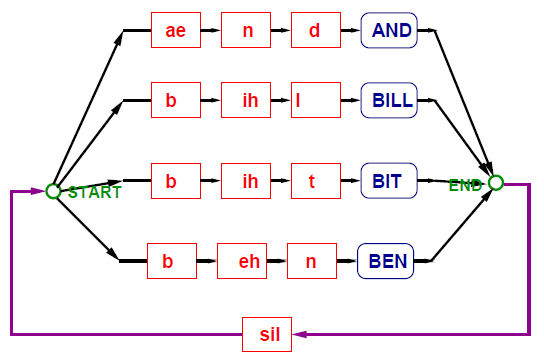
However, this parallel organisation is suboptimal. Many words start with the same phoneme, and consequently the same model at the start. Thus, some parallel branches can be merged into a tree-like structure.

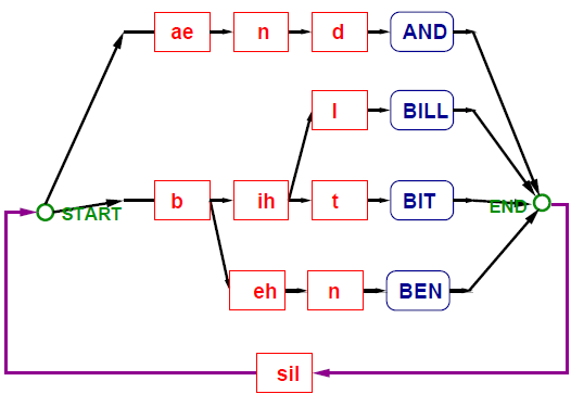
This reduction in the number of models in the network has a direct impact on the computational complexity. For the token passing algorithm, each state in the network has to hold exactly one token. Each token requires propagation and thus incurs computational cost, which can be lessened by reducing the number of models in this way.

Monophone models normally have inferior performance to triphone models. For word-internal models, these networks can be constructed similar to the monophone models, but the benefits of tree organisation for word-internal triphones are not as great.

For cross-word triphone models, which offer further benefits over word-internal triphone models, the construction of the network is more complex. Words will have multiple start and end nodes depending on the phonemes at the start of the next loop. This also has the issue of not having all word-end nodes connected to all word-start nodes.

To cope with this, the token passing algorithm must be modified so that the "best word" decision now has to be made for each set of links for entering one particular word.

We must also consider the impact our language model has on our pronunciation organisation. For n-grams, the search space is vastly increased, as the language model probabilities can be interpreted as transition probabilities in a huge composite model between word starts and ends.

Alternate methods must be found to deal with this vastly increased search space. These use appropriate methods for constraining the search, but has the downside of not necessarily finding the best word sequence.

Beam Search

In speaker clustering, a large number of model sets are generated, each one corresponding to a different speaker. The adaptation problem then reduces to deciding which model set the current speaker belongs to - a speaker identification problem.

In practice, it is not possible to generate a model set for every individual speaker, due to limitations of training data. Speakers are therefore clustered into similar speaker groups, and model sets are trained for these speaker groups.

During adaptation, the most suitable speaker group is selected. Hence, the speaker adaptation problem is separated into a clustering task and a classification problem.

In practice, this approach is problematic. The spectral variation of speakers, even within a cluster, may be large. Additionally, new speakers may not be well represented by the training set of speakers, and it is assumed that the differences between speakers are uniform across a model set.

Improved techniques such as eigenvoices or cluser adaptive models exist.

In feature normalisation, parameters in the extracted features are adjusted to optimal values for a certain speaker. The aim is to lower or even remove the inter-speaker variability of speech signals.

With this approach, normally high efficiency is reached, but due to the small number of parameters, results rarely reach SD performance.

The most well known techniques for feature normalisation are vocal-tract length normalisation, where the length of the vocal tract is estimated, and the spectral shifts calculated accordingly, and linear cepstral transformation, where a general linear transformation of the cepstral features is used.

Algorithmically, both schemes are related - vocal-tract length normalisation can be approximated by linear transforms.

Vocal-Tract Length Normalisation

Model-based adaptation approaches have become increasingly popular. The aim is now to alter the parameters of, for example, a speaker independent model set to be more representative of a particular speaker.

Two approaches are common here: maximum a-posteriori (MAP) approaches, which have been used extensively for speaker adaptation, and smoothing; and linear regression, where a linear transformation is applied to the Gaussian mean (and possibly variance) parameters.

One problem that occurs with these model adaptation approaches is that of unobserved Gaussians - i.e., when there are no frames of adaptation data that correspond to a particular part of the model. This is a more general problem with speaker adaptation, as wehen dealing with small amounts of adaptation data, few Gaussians will be observed in the adaptation data.

MAP Estimation

Least Squares Linear Regression

Maximum Likelihood Linear Regression

For linguistic analysis, the input is human readable text (potentially with special characters and abbreviations), and the output is a high level description of the speech sounds to be generated.

The initial stages of the process are designed to diambiguate the sense of each word or character, and the following stages deal with the translation of words, together with additional syntactically/semantically derived information, into a compact description of the sounds to be generated.

The stages in linguistic analysis are: text normalisation, morphological analysis, syntactic analysis, pronunciation generation, intonation, and phonological analysis.

Text Normalisation

Morphological Analysis

Syntactic Analysis

Pronunciation Generation

Intonation

Phonological Analysis

The synthesis stage of a TTS system must convert the allophone symbol sequence into a continuous speech waveform, and apply the correct innotation.

Common forms of synthesis include formant-based, articulatory and concatenative. Formant-based synthesisers can be either parallel or serial, and vocal tract filter is formed by combining a number of resonances. Articulatory synthesis attempts to model the speech production system, and models of the articulators and vocal cords are used - the original "speech machine". Concatenative synthesis explicitly uses synthesis units - representative examples of each unit is stored and used for synthesis.

Many of these systems make use of the source-filter model of speech production. The source-filter model represents the vocal tract in the form of a time-varying filter, and assumes a binary selection between two forms of excitation sources: a noise and a pulse generator. Excitation is modelled as either a train of impulses, or by noise. The vocal tract filter has to be modified frequently (e.g., every 10 ms)

The excitation is described by F0 and energy alone, but the parameters of the filter can take many forms, such as descriptive using formants, or signal representative using spectral representations.

Formant Synthesis

Articulatory Synthesis

Concatenative Synthesis