What is Computer Graphics?
Angel c.1
Computer graphics is concerned with all aspects of producing pictures or images using a computer; the ultimate aim is to represent an imagined world as a computer program.
A Brief History
- pre-1950s - Crude hardplots
- 1950s - CRT displays (e.g., as seen in early RADAR implementations)
- 1963 - Sutherland's sketch pad
- 1960s - The rise of CAD
- 1970s - Introduction of APIs and standards
- 1980s - Rise of PCs lead to GUIs and multimedia
- 1990s - Visualisation, rise of the Internet, WWW, Java, VRML
Computer graphics have many applications, such as displaying information as in meterology, medical uses and GIS; design as with CAD/CAM and VLSI as well as simulation, such as virtual reality, pilot training and games.
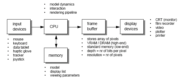
Graphics systems are raster based - represented as an array of picture elements known as pixels stored in a frame buffer. Vector based systems on the other hand work by following a set of instructions and outputing the results. Raster based systems are faster, but require more memory.
Graphics are ultimately about controlling pixels, but we use primitives to abstract away from the pixels.
Mathematical Basics
Angel c.4
We can consider some mathematical basics when dealing with computer graphics. We can consider points - locations in space specified by coordinates, lines - which join two points, a convex hull - the minimum set which includes all points and the line segments connecting any two of them, and a convex object - where any point lying on the line segment connecting any two points in the object is also in the object.
In computer graphics, we also use vectors for relative positions in space, orrientation of surfaces and the behaviour of light. We can also use them for trajectories of dynamics and operations. A vector is a n-tuple of real numbers, and addition and scalar multiplication is done quite straight forwardly by either adding each individual term to the corresponding one in another vector, or by multipying each individual element by a scalar.
Trigonometry (sine, cosine, tangent, etc) is also used to calculate directions of vectors and orrientations of planes.
We can also use the dot (inner) product of vectors, where a ∧ b = |a||b|cos θ. The product can be calculated as a ∧ b = x1y1 + ... + xnyn. We can use this to figure the Euclidean distance of a point (x, y) from the origin d = √ (and similarly for n-dimensional space).
The dot product can also be used for normallising a vector.v′ = v/||v|| is a unit vector, it has a length of 1. The angle between the vectors v and w can be expressed as: cos-1((v ∧ w)/(||v|| ||w||)). If the dot product of two vectors v and w is 0, it means that they are perpendicular.
Matrices
Matrices are arrays of numbers indexed by row and column, starting from 1. We can consider vectors as n × 1 matrix. If A is an n × m matrix and B is a m × p matrix, then A ∧ B is defined as a matrix of dimension n × p. An entity of A ∧ B is cij = Σms = 1 aisbsj.
The identity matrix is the matrix where Ixy = 1, if x = y, otherwise 0, and transposing a n × m matrix gives an m × n matrix: Aij = A′ji.
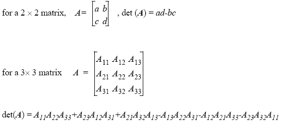
A determinant (det A) is used in finding the inverse of a matrix. If det A = 0, it means that A is singular and has no inverse.
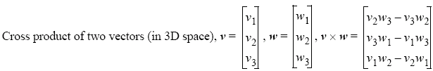
Given two vectors v and w we can construct a third vector u = w × v which is perpendicular on both v and w, we call this the cross product.
Planes
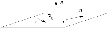
Three points not in a line determine a unique plane. Three edges forming a triangle determine a plane. A plane can be determined by point P0 and two unparalleled vectors u and v.
The equation of a plane can be expressed as T(α, β) = P0 + αu + βv. An equation of a plane given the plane normal n: n ∧ (P - P0)
Planes are used for modelling faces of objects by joinin edges and vertices. In this case, their service normals are used to represent shading and other more complex lumination phenomena such as ray tracing. You can then visualise correspondingly the texture that is applied onto objects. You can also model the visualisation system with planes, and they constitute the basis for more complex surfaces (e.g., curved surfaces come from patches that are planar in nature).
Transformations
There are three fundamental transformations in computer graphics, which can be expressed using vectors and matrices.
![]()
However, we now have the problem that translation can not be expressed using matrix multiplication, so we move from from cartesian to homogenuous (projective) coordinate space. Each affine transformationis represented by a 4 × 4 matrix within a reference system (frame). The point/vector (x, y) becomes (x, y, w), so (x1, y1, w1) = (x2, y2, w2) if x1/w1 = x2/w2 and y1/w1 = y2/w2. This division by w is called homogenising the point. When w = 0, we can consider the points to be at infinity.
Now we are working in homogenuous space, we can apply uniform treatment:
![]()
Shearing can be used to distort the shape of an object - we shear along the x axis when we pull the top to the right and the bottom to the left. We can also shear along the y axis.
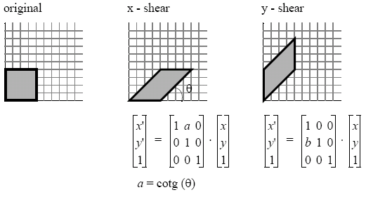
Transformations of a given kind can be composed in sequence. Translations can be used to apply transformations at arbitrary points. When composing different translations, the last translation to be applied to the matrix is applied first, and then backwards from that. Transformations are generally associative, but have non-commutativity.
Special orthogonal matrices can be used to simplify calculations for rigid body transformations:
![]()
3D Transformations
For 3D transformations, the same principles apply, but now in a 4D homogenuous space. However, rotation now has to be defined with respect to a specific axis.
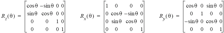
However, if we want to rotate a cube with the centre in P0 around an axis v with the angle β. The unit vector v has the property cos2Φx + cos2Φy + cos2Φx = 1. We can denote the coordinates of v by αx = cosΦx, αy = cosΦy and αz = cosΦz. We should decompose all the necessary rotations into rotations about the coordinate axes.
Graphics often utilise multiple coordinate spaces. We can express this as P(i), as the representation of P in coordinate system i. To translate between the two systems, we apply the matrix Mi←j, as the transformation from system j to system i
Primitives
Angel c.2
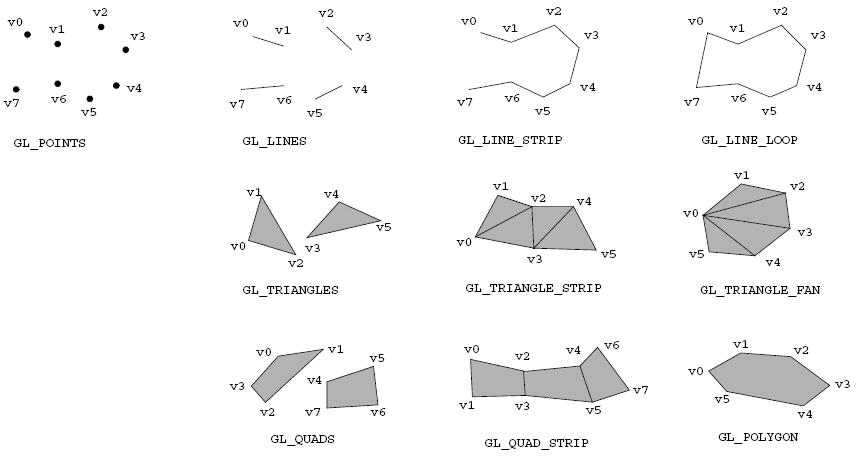
In OpenGL, we specify primitives by declaring glBegin(mode);, followed by a specification of the vertices and other properties, and then we end the primitive definition with glEnd();. The mode in this case is a specification of which primitive we want to define, such as:
Examples are in
lecture slides.
And vertices can be specified using glVertexNT(TYPE c1, TYPE c2, ..., TYPE cn);, where N is the number of dimensions of the vertex (2, 3 or 4) and T is a character indicating the data type, s for short, i for integer, f for float and d for double. Alternatively, the vertex arguments could be passed as an array using glVertexNTv(TYPE coords[]);.
We can also consider other primitives, such as curves, circles and ellipses, which are typically specified by a bounding box (an extent), a start angle and an end angle, although variations exist which use the centre and a radius, different implementations use radians vs. degrees and allow the orrientation of the bounding box to be changed. NURBS are also common and are what OpenGL uses. Simple curves are non-existant in OpenGL and must be defined using quadrics.
When talking about points, we can consider the convex hull - the minimum set which includes all the points and the line segments connecting any two of them. The convex object consists of any point lying on the line segment connecting any two points in the object.
We can also consider text as a primitive. Text comes in two types, stroke fonts (vector), where each character is defined in terms of lines, curves, etc... Stroke fonts are fairly easy to manipulate (scaling and rotation, etc), but this takes CPU time and memory. Bitmap (raster) fonts are where each character is represented by a bitmap. Scaling is implemented by replicating pixels as blocks of pixels, which gives a block appearance. Text primitives give you control of attributes such as type, colour and geometrical parameters and typically require a position and a string of characters at the very least.
OpenGL support for text is minimal, so GLUT services are used, such as glutBitmapCharacter(); and glutStrokeCharacter();.
Some primitives are used to define areas, so a decision needs to be made on whether or not these area-definining primitives need to be filled or outlined. In OpenGL, polygonal primitives are shaded, and explicit control is given over the edge presence. More complicated effects can be accomplished by texturing. This fill attribute may allow solid fills, opaque and transparent bitmaps and pixmaps.
A final primitive to consider is that of canvases. It is often useful to have multiple canvases, which can be on- or off-screen, and there consists of the default canvas, and a concept of a current canvas. Canvases allow us to save or restore image data, and support buffering and have a cache for bitmap fonts. The OpenGL approach to canvases uses special-purpose buffers, double buffering and display lists.
Curves and Surfaces
Up until now, curves and surfaces have been rendered as polylines and polygonal meshes, however we can use piecewise polynomial functions and patches to represent more accurate curves and curved surfaces.
Parametric equations (one for each axis) are used to represent these, where each section of a curve is a parametric polynomial. Cubic polynomials are widely used due to having an end-point and gradient continuity, as well as being the lowest degree polynomial that is non-planar. Curve classes are used due to the constraints used to identify them (points, gradients, etc).
Parametric polynomials of a low degree are prefered as this gives us a local control of shape, they have smoothness and continuity and derivatives can be evaluated. They are fairly stable and can be rendered easily too - small changes in the input should only produce small changes in the output.
The points are called curve and segment points.
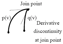
We can consider two types of geometric continuity of 2 segments:
- segments join (G0)
- tangent directions are equal at the join point, but magnitudes do not have to be (G1)
We can consider three properties of parametric continuity:
- all three parameters are equal at the join point (C0)
- G1 (only required if curves have to be smooth) and the magnitudes of the tangent vectors are equal (C1)
- The direction and magnitude of ∀i, i ∈ N, 1 ≤ i ≤ n, di/dtiQ(t) are equal at the join point (Cn - however n > 1 is only relevant for certain modelling contexts, e.g., fluid dynamics).
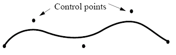
Hermite Curves
Hermite curves are specified using two end-points and the gradients at the end points, and these characteristics specify the Hermite geometry vector. The end points and tangents should allow easy interactive editing of the curve.
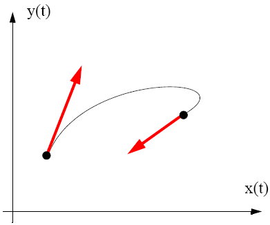
By changing the magnitude of the tangent, we can change the curve whilst maintaining G1 consistency.
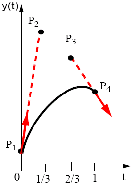
Bézier Curves
Parametric gradients are not intuitive, so an alternative is to use 4 points, of which 2 are interpolated and 2 which are approximated. We can then figure out G1 = dQ(0)/dt = 3(P2 - P1) and G2 = dQ(1)/dt = 3(P4 - P3).
Bézier curves and surfaces are implemented in OpenGL. To use them, we need a one-dimensional evaluator to compute Bernstein polynomials. One dimensional evaluators are defined using glMap1f(type, u_min, u_max, stride, order, point_array), where type is the type of objects to evaluate (points, colours, normals, etc), u_min and u_max are the range of t, stride is the number of floating point values to advance between control points, order specifies the number of control points and point_array is a pointer to the first co-ordinate of the first control point. An example implementation of this may be:
GLfloat control_points[4][3] = {{-4.0, -4.0, 0.0} {-2.0, 4.0, 0.0} {2.0, -4.0, 0.0} {4.0, 4.0, 0.0}};
glMap1f(GL_MAP1_VERTEX3, 0.0, 1.0, 3, 4, &control_points[0][0]);
glEnable(GL_MAP1_VERTEX3);
glBegin(GL_LINE_STRIP);
for (i=0;i<=30;i++) glEvalCoord1f((GLfloat) i/30.0);
glEnd();
To implement Bézier surfaces, the glMap2f(type, u_min1, u_max1, stride1, order1, u_min2, u_max2, stride2, order2, point_array) function can be used, along with glEvalCoord2f(), or you can use glMapGrid2f() and glEvalMesh2().
B-splines
Bézier curves and patches are widely used, however they have the problem of only giving C0 continuity at the join points. B-spline curves can be used to obtain C2 continuity at the join points with a cubic.
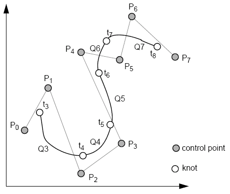
The B-spline consists of control points (Pi), cubic poly segments (Q3, Q4, ..., Qm) and Qi is defined on ti ≤ t ≤ ti + 1, 3 ≤ i ≤ m. Control points affect four segments.
Knots lay between Qi and Qi + 1 at ti (the knot value). t3 and tm + 1 are end knots, and are equally spaced (uniform), so ti + 1 = ti + 1 (therefore the blending function is the same for all segments).
We can call these curves non-rational to distinguish it from the rational cubic curves (a ratio of polynomials).
Another variety of B-splines also exist - non-uniform non-rational B-splines. Here, the spacing of the knots (in parameter space) is specified by a knot vector (the value of the parameter at the segment joins).
The table below compares Bézier curves with uniform B-splines:
| Representation | Bézier Curves | Uniform B-splines |
|---|---|---|
| Compute a new spline | Every 3 points | Every new point |
| Smoothness | Good | Very good |
| Each control point affects: | The entire curve | Maximum four curve segments |
| Continuity | C0 and C1 (if additional constraints are imposed) | C0, C1 and C2 |
| Complexity of a curve segment | High | Low |
| Number of basis functions | Four | Four |
| Interpolation properties | Interpolates the end control points | May not interpolate any point |
| The convex hull of the control points | Contains the curve | Contains the curve |
| Sum of the basis functions | Equal to one | Equal to one |
| Affine transformation to its control point representation | Transforms the curve accordingly | Transforms the curve accordingly |
Processing Pipeline
Angel c.2
We can consider the processing pipeling as: Modelling → Geometric Processing → Rasterisation → Display, and we can further break down Geometric Processing to Transformation (4×4 matrices which transform between two co-ordinate systems) → Clipping (Generated by a limited angle of view) → Projecting (4×4 matrices describing the view angle). This can be implemented using custom VLSI circuits, or with further refinement using things such as shaders, etc...
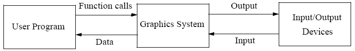
Pipelines introduce latency, delays for a single datum to pass through the system. The interface between an application program and the graphics systems can be specified using a set of functions that reside in a graphics library.
These APIs are device independent, and provide high-level facilities such as modelling primitives, scene storage, control over the rendering pipeline and event management.
We can consider the following general principles and structures:
- Primitive functions - define low level objects and atomic entities
- Attributes - these govern the way objects are displayed
- Viewing functions - specifying the synthetic camera
- Transformations - geometrical transformations (translation, rotation, scaling, etc)
- Input functions - functions used to input data from the mouse, keyboard, etc
- Control functions - responsible for communications with the windowing system
OpenGL Interface
In an X Windows system, the OpenGL system could be represented as follows:
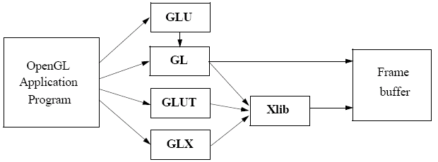
GL is our basic graphics library and consists of all the primitive functions, GLU is the graphics utility library and uses GL, GLUT is the graphics utility library toolkit and interfaces with the windowing system. The library is constantly expanding. The final component, GLX for X Windows, or on Microsoft Windows wgl communicates with the X windowing system, or the Windows window subsystem.
Modelling
Angel c.9
There are two different kinds of modelling - a domain model and a graphical model. The domain model is a high-level abstraction of the objects and normally refer to objects, whereas the graphical model is a low-level implementation and refers to points, vertices, polygons, etc...
When we model, we can do it in two modes - in an immediate mode, where no record is kept of primitives or the attributes, and the image is regenerated by respecifying the primitives - and a retained mode, where a graphical model is stored in a data structure (called a display list in OpenGL) and a scene database is stored.
In OpenGL, we use display lists, which are a cache of commands (not an interactive database - once it has been created, it can not be altered). Display lists can be created in two modes - GL_COMPILE and GL_COMPILE_AND_EXECUTE, where the display list is executed as it is declared.
A modelling coordinate system is used to define individual objects (located at the origin, axis aligned), and then objects are combined within a world coordinate system.
To simplify complex problems, we can encapsulate scenes into 'self-contained' packages, which localise changes and allow reuse. This is typically done with either display lists, or for more complex display lists (as you can not have display lists within a display list ), with procedures that call multiple display lists. This in itself is not fundamental to modelling, but has a lot of efficiency increases.
In OpenGL, you create a display list using glGenLists(1), which will return a GLuint (which will be 0 if a failure has occured), and the actual contents of the list are generated in between glNewList(GLuint list, mode) and glEndList(). They are then called using glCallList(list) and free'd with glDeleteList(list, 1). glIsList(list) is used to check for the existance of a list.
Most things can be cached into a display list (with the exception of other display lists), however things that change a clients state (such a GLUT windowing commands) are executed immediately.
Matrices
Matrices are used to isolate different transformations (for example, for each individual model) from different transformations. In OpenGL, matrices are stored on a stack, and they can be manipulated with:
- glPushMatrix() - this is a 'double up' push, where the current matrix is pushed on to the top of the stack, but is still available as the current matrix
- glPopMatrix() - this replaces the current matrix with the one on the top of the stack
- glLoadMatrix(GLfloat *M) - replaces the current matrix with the matrix M, a special version of this, glLoadIdentity() loads the identity matrix
- glTranslate(), glRotate(), glScale(), glMultMatrix(GLfloat *M) - in each case the new matrix is premultiplied by the current matrix and the result replaces the current matrix.
Stack based architectures are used by most graphics system, as they are ideally suited for the recursive data structures used in modelling.
Due to the way matrix multiplication works, actions on the matrix start from the one most recently applied and move backwards in the reverse order to how they were applied.
An OpenGL programmer must manage the matrix and attribute stacks explicitly!
Attributes
Similar to a matrix stack, the attribute stack can be manipulated to hold attributes that can be expensive to set up and reset when rendering a model.
Attributes tend to be organised into attribute groups, and settings of selected groups (specified by bitmasks) can be pushed/popped. glPushAttrib(GLbitfield bitmask) and glPopAttrib() work in the same way as the matrix stack. One of the most common bitmasks is GL_ALL_ATTRIB_BITS, but more can be found in the manuals.
A version also exists for networked systems: glPushClientAttrib(GLbitfield bitmask) and glPopClientAttrib().
Materials
Three dimensional structures are perceived by how different surfaces reflect light. Surfaces may be modelled using glMaterialfv(surfaces, what, *values), where surfaces is which surfaces are to be manipulated (i.e., just the front of a polygon with GL_FRONT or both sides with GL_FRONT_AND_BACK) what is the material attribute to be manipulated (e.g., GL_AMBIENT_AND_DIFFUSE for lighting and GL_SHININESS for shininess). For single values, glMaterialf(surfaces, what, v) can be used.
An alternative is just simply colour the materials using glColorMaterial(GL_FRONT_AND_BACK, GL_AMBIENT_AND_DIFFUSE) and then wrapping the objects to be created with glEnable(GL_COLOR_MATERIAL) and glDisable(GL_COLOR_MATERIAL), and then using standard glColor3f() commands.
Lighting
Lighting effects require at least one light source, and OpenGL allows at least 8 specified by GL_LIGHTn.
Global lighting is enabled using glEnable(GL_LIGHTING) and then specific lights can be turned on or off using glEnable(GL_LIGHTn) and glDisable() respectively.
The attributes of lights are specified using glLightfv(GL_LIGHTn, attribute, *value), where attribute is the attribute of the light to be set up (e.g., GL_AMBIENT, GL_DIFFUSE, GL_POSITION, GL_SPECULAR).
Ambient Sources
Ambient sources have a diffused, non-directional source of light. The intensity of the ambient light is the same at every point on the surface - it is the intensity of the sources mulitplied by some ambient reflection coefficient.
This is defined in OpenGL with glMaterial{if}v(GLenum face, GLenum pname, TYPE *params);. face is either GL_FRONT, GL_BACK or GL_FRONT_AND_BACK, pname is a parameter name, and in this case we use GL_AMBIENT, and params specifies a pointer to the value or values that pname is set to, and this is applied to each generated vertex.
Objects and surfaces are characterised by a coefficients for each colour. This is an empirical model that is not found in reality.
Spotlights
Spotlights are based on Warn's model, and simulate studio lighting effects. The itensity at a point depends on the direction, and flaps ("barn doors") confine effects sharply. Spotlights are often modelled as a light source in a cone.
Spotlights in OpenGL are implemented using the GL_SPOT_CUTOFF and GL_SPOT_EXPONENT parameters to glLight.
Graphics File Formats
Most graphics programming is done in modelling applications which output the model in a file format. Common file formats include:
- VRML (Virtual Reality Modelling Language) - an open standard written in a text form
- RasMol - a domain modelling language used in molecular chemistry, in which the file contain a text description of the coordinates of atoms and bonds in a model
- 3D Studio - a proprietary file format developed by AutoDesk that is very common in industry
Solid Object Modelling
Angel c.9.10
When we model with solid objects, rather than surfaces only, we can do boolean set operations on the objects - union, intersection and subtraction. When we apply these to volumes, these operations are not closed, as they can yield points, lines and planes, so we only consider regularised boolean set operations, which always yield volumes, so the intersection of two cubes sharing an edge is null.
It is difficult to define boolean set operations with primitive instancing, this is where objects are defined as a single primitive geometric object and is scaled, translated and rotated into the world (as we have been doing with display lists in OpenGL). Primitive instancing is simple to implement, however.
Sweep Representations
This is where an area is swept along a specified trajectory in space. We can consider this as either extrusion, where a 2D area follows a path normal to the area and rotational sweeps, where an area is rotated about an axis (however, these do not always produce volumes).
When sweeping, if we sweep a 3D object, this will always guarantee a volume, and in the process of sweeping may change the shape, size and orientation of the object. Trajectories can be complex (e.g., following a NURBS path), and it is not clear what the representational power of a sweep is (what volume operations can we perform?). We typically use these as input to other representations.
Constructive Solid Geometry
Constructive solid geometry is based on the construction of simple primitives. We combine these primitives using boolean set operations and explicitly store this in the constructive solid geometry representation, where tree nodes are operators (and, or or diff) and leaves are primitives. The primitives themselves can be simple solids (guaranteeing closed volumes or an empty result), or non bounded solids - half-spaces, which provide efficiency. To compute the volume, we can use traversal.
Boundary Representations
Boundary representations (B-reps) are one of the simplest representations of solids. They require planar polygonal faces, and are historically implemented through traversing faces and connected edges, due to the vector graphics for which their efficiency is aimed.
B-reps require represented objects to be two-manifold. An object is two manifold if it is guaranteed that only two faces join at an edge, i.e., a surface must be either of the forms shown below, not both at the same time, which would cause us to move in to hyperspace.
B-reps consist of a vertex table with x, y and z co-ordinates, an edge table consisting of a pair of the two vertices connected by an edge and a face table consisting of a list of which edges denote a face.
Winged-edge representation is a common representation of b-reps, where each edge has pointers to its vertices, the two faces sharing the edge and to four of the edge emanating from it. Using winged-edge representation, we can compute adjacency relationships between faces, edges and vertices in a constant time.
Spatial partitioning representations are a class of representations that work by decomposing space into regions that are labelled as being inside or outside the solid being modelled. There are three types to consider.
Spatial Occupancy Enumerations
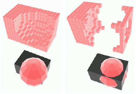
These are voxel based systems, where the material is represented by a succession of small cubes like pixels in a display. The precision of the scene is the size of the voxel, the more voxels you have, you have an increase in precision, but at the expense of memory and computation increase (Ο(n3)).
This approach is good for fast clearance checking in CAD, although many optimisations can be made. Additionally, having a good level of precision tends to cause problems, and no analytic form exists for faces or surfaces. It is fairly easy to compute the volume, however, as volume = voxel volume × number of voxels.
Quadtrees and Octrees
Quadtrees is spatial occupancy enumeration with an adaptive resolution - pixels are not divided when they are either empty or fully occupied. Net compression occurs, and it seems likely that intersection, union and difference operations are easy to perform.
Octrees are the quadtree principle extended to be in three dimensions, so a division of a voxel now produces 8 equal voxels. They can easily be generated from other representations and are rendered from front to back. They are logically equivalent to quadtrees so boolean operations are easily possible.
Representing octrees in a tree form has a high memory cost, so we can use various linear encodings. Octrees are commonly used to partition worldspace for rendering optimisation and for occlusion culling.
Binary Space Partitioning Trees
Binary space partitioning (BSP) trees are an elegant and simple representation that deals only with surfaces, not volumes. It does have a potentially high memory overhead, but boolean operations and point classification are easy to compute.
Physics
Angel c.11
Fractals
The basic characteristics of a fractal are that they have infinite detail at any point, exhibit self similarity and are defined procedurally. They can be applied to generate terrains, clouds, plants and flowers. Fractals can be classified into two basic types, self-similar (has statistical self-similarity) and self-affine (exact self-similarity).
If we are dealing with objects defined in three dimensional space, then the euclidian dimension (De) of an object is the number of variables required the specify the points in the object. In 3D space, this is always 3. The topological dimension (Dt) of an object is the minimum number of intersections of spheres needed to ensure coverage of the object. For discrete points, Dt is 0; for lines, Dt is 1; for planes, Dt is 2; and for volumes, Dt is 3.
The similarity dimension Ds is a measure of the way an object scales with respect to measuring a lengthε. In general, this is NεD = 1, hence Ds = log(N)/log(1/ε).
Cantor Set
One famous fractal is the Cantor Set (sometimes called Cantor Dust) derived by Georg Cantor. It consists of discrete points on an interval of a real line, but has as many points as there are in an interval. In general, the interval is divided into 2k segments which in the limit k = ∞ gives 2N0 discrete points. Since the points are discrete, the topological dimension Dt = 0, but we can consider the similarity dimension to be Ds = log(2)/log(3) = 0.6309.
Kock Curve
Like the Cantor Set, the Kock curve is formed from an interval of the real line, but it is infinitely long, continuous and not differentiable.
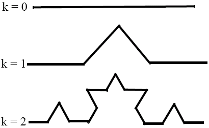
As we have a curve, the topological dimension Dt = 1, but the similarity dimension Ds = log(4)/log(3) = 1.2618.
A fractal is defined as any curve for which the similarity dimension is greater than the topological dimension. Other definitions do exist, e.g., when the Hausdroff dimension is greater than the topological dimension (Mandelbrot, 1982), but this fails for curves which contain loops. Another defintion is any self-similar curve (Feder, 1988), but this includes straight lines, where are exactly self-affine.
Fractals are problematic, as they take a large amount of computational time to render and are quite difficult to control. An alternative method that could be used is random midpoint displacement, which is faster, but less realistic. In random midpoint displacement, the midpoint of a straight-line segment a-b is displaced by r, a value chosen by Gaussian distribution, a mean or a variance.
Another way to represent fractals is as self-squaring fractals. If you take a point x + iy in complex space and repeatedly apply the transformation zn + 1 = zn2 + c. This will either diverge to infinity, converge on a fixed limit (an attractor) or remain on the boundary of an object - the Julia set. The Julia set may be disconnected depending on the control factor c). A special set known as the Mandelbrot set is all values of c that give a connected Julia set. Sets are found by probing of sample points and inverse transformation.
Shape Grammars
Shape grammars are production rules for generating and transforming shapes. They are especially useful for plants and patterns. Strings can be interpreted as a sequence of drawing commands, e.g., F - forward, L - left, R - right some angle.
Particle Systems
Particle systems can be used to model objects with fluid-like properties, such as smoke, fish clouds, waterfalls, groups of animals, etc...
In particle systems, a large number of particles are generated randomly, and objects are rendered as very small shapes. Parameters (e.g., trajectory, color, etc) vary and evolution is controlled by simple laws. Particles eventually spawn or are deleted. One way of dealing with particle systems is to start with organised particles and then disintegrate the object.
Constraints allow aspects of real world behaviour to be added to an evolving particle system, e.g., particles may bounce off a surface or be deflected by some field. Two forms of constraints exist: hard constraints, which must be enforced, e.g., a surface off which particles must bounce, these are difficult to implement as new behaviours and detectors must be set up; and soft constraints, which may be breached - these are usually implemented using penalty functions that are dependent on the magnitude of the breach of the constraint. They are often simpler to implement and can be very efficiently be described in terms of energy functions similar to potential energy.
Physically Based Models
Physically based models can be used to model the behaviour of non-rigid objects (e.g., clothing, deforming materials, muscles, fat, etc...), and the model represents interplay between external and internal forces.
Key Framing
Key framing is the process of animating objects based on position and orientation at key frames. This "in betweening" generates auxilary frames using motion paths - they can be specified explicitly (e.g., using lines and splines) or generated procedurally (such as using a physics based model). Complexities can be caused by objects changing shape; objects may gain and lose vertices, edges and polygons, so we can consider a general form of key-framing as morphing (metamorphosis).
Animation paths between key frames can be given by a curve-fitting techniques, which allows us to support acceleration. We can use an equal time spacing with in-betweens for constant speed, but for acceleration, we want time spacing between in betweens to increase, so an acceleration function (typically trigonometric) is used to map in between numbers to times.
Cameras
Angel c.1
Images are formed by light reflecting off objects and being observed by a camera (which could include the human eye).
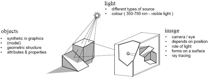
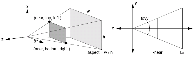
In simple cameras, the image consists of projections of points, and with the pinhole model, we can assume an infinite depth of field. We can also consider the field of view, which maps points to points and the angle of view, which depends on variables d and h as in the diagram below.
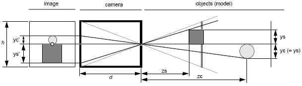
ys′ = -ys/(zs/d) and yc′ = -yc/(zc/d).
We can also consider synthetic cameras:
Viewing Transformations
For a more in-depth
treatment, see lecture 6.
Angel c.5
Viewing determines how a 3D model is mapped to a 2D image.
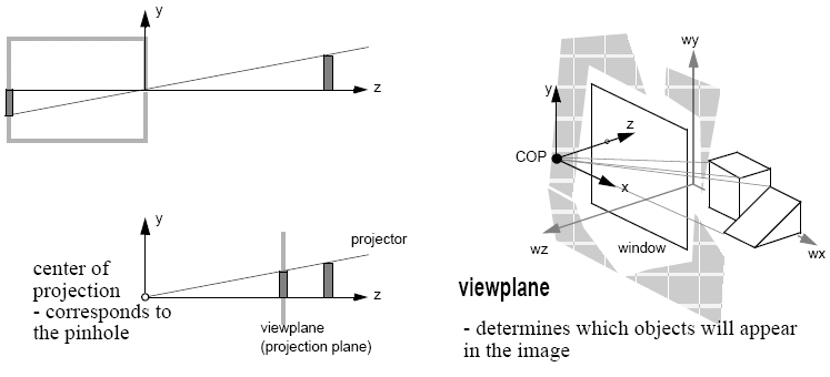
In the real world, we pick up the object, position it and then look at it, however in computer graphics, objects are positioned in a fixed frame and the viewer then moves to an appropriate position in order to achieve the desired view - this is achieved using a synthetic camera model and viewing parameters.
The important concepts in viewing transformations are the projection plane (the viewplane) and projectors - straight projection rays from the centre of projection. The two different forms of projection are perspective (the distance from the centre of projection to the view plane is finite - as occurs in the natural world), and parallel, where the distance from the centre of projection to the view plane is infinite, so the result is determined by the direction of projection.
With perspective projection, lines not parallel to the viewplane converge to a vanishing point. The principal vanishing point is for lines parallel to a principal axis, and an important characteristic is the number of vanishing points.
With parallel projection, the centre of projection is at infinity, and the alignment of the viewplane is either at the axes, or in the direction of projection.
We can define a view reference coordinate system, where the world coordinates are relative to the camera, rather than the origin. In this system, we have many parameters, such as:
- location of the viewplane
- window within the viewplane
- projection type
- projection reference point (prp)
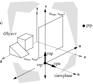
The viewplane also has parameters such as view reference point (vrp), the viewplane normal (vpn) and the view up vector (vuv), and the window has width and height defined.
In the perspective space, the prp becomes the centre of projection and in the parallel case we have the concept of a window centre and the direction of projection is the vector from prp to the window centre. If the direction of projection and vpn are parallel, this gives us an orthographic projection.
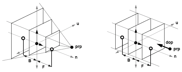
Clipping Planes
The viewplane window clips the sides of images, so we can also limit the depth of view by using front and back clipping planes. We can use this to implement depth cueing, focusing on objects of interest and culling artefacts (both near and far). To create a clipping plane, we need a distance along the n axis - all planes are created parallel to the viewplane. In perspective projection, if we have negative distances (behind the centre of projection), we see objects upside down. Nothing in the plane of the centre of projection can be seen.
With clipping planes, we can now consider view volumes. For perspective views, we have a truncated pyramid (a frustrum), but in the parallel view, we get a rectangular solid:
In OpenGL, we have a current transformation matrix (CTM) that operates on all geometry. There are two components to this: a model view matrix and a projection matrix. The model view matrix addresses modelling transformations and camera position and the projection matrix deals with 3D to 2D projection. OpenGL transformations can be applied to either matrix, but we need to explicitly select the mode using glMatrixMode(GL_MODELVIEW) or glMatrixMode(GL_PROJECTION). Normally, we leave it in model-view mode, however.
We can also explicitly manipulate the matrix using glLoadIdentity(), glLoadMatrix{fd}(const TYPE *m), glMultMatrix{fd}(const TYPE *m). We can also implicitely construct a matrix using gluLookAt(GLdouble ex, GLdouble ey, GLdouble ez, GLdouble cx, GLdouble cy, GLdouble cz, GLdouble ux, GLdouble uy, GLdouble uz). e refers to the position of the eye, c to the point being looked at and u tells you which way is up.
For perspection projection, the projection matrix can be defined using transformations, but it is much simpler to use 'pre-packaged' operators: glFrustrum(GLdouble left, GLdouble right, GLdouble bottom, GLdouble top, GLdouble near, GLdouble far) and gluPerspective(GLdouble fovy, GLdouble aspect, GLdouble near, GLdouble far).
For orthographic projection, the parameters define a rectanglar view volume: glOrtho(GLdouble left, GLdouble right, GLdouble bottom, GLdouble top, GLdouble near, GLdouble far). A simplified form for 2D graphics also exists: gluOrtho2D(GLdouble left, GLdouble right, GLdouble bottom, GLdouble top).
Projection transformations map a scene into a canonical view volume (CVV). OpenGL maps into the full CVV given by the function glOrtho(-1.0, 1.0, -1.0, 1.0, -1.0, 1.0).
Viewport transformations locates the viewport in the output window. Distortion may occur if aspect ratios of the view volume and the viewport differ. The viewport and projection matrices may need to be reset after the window is resized.
![]()
Visible Surface Determination
Angel c.5.6, 8.8
Visible surface determination is all about figuring out what is visible, and is based on vector mathematics.
Coherence is the degree to which parts of an environment exhibit self similarity, and it can be used to accelerate graphics by allowing simpler calculations or allowing them to be reused. Types of coherence are:
- Object coherence - if objects are totally seperate, they may be handled at the object level, rather than the polygon level
- Face coherence - properties change smoothly across faces, so solutions can be modified across a face
- Edge coherence - an edge visibly changes when it penetrates or passes behind a surface
- Implied edge coherence - when one polygon penetrates another, the line of intersection can be determined from the edge intersections
- Scan-line coherence - typically, there is little difference between scan lines
- Area coherence - adjacent pixels are often covered by the same polygon face
- Depth coherence - adjacent parts of a surface have similar depth values
- Frame coherence - in animation, there is often little difference from frame to frame
Two ways of solving this include using image precision and object precision. In image precision, an object is found for each pixel, and this has complexity Ο(np), where n is the number of objects and p is the number of pixels , whereas for object precision, for each object the pixels that represent it are displayed, and then it is discovered whether said pixel is obscured, and this has complexity Ο(n2), so this method is good when p > n, or in other words, when there are not many pixels.
One simple way of implementing object precision is using extents and bounding boxes. With bounding boxes, a box is drawn around each polygon/object and if any of the boxes intersect, then we know we need to check for occlusion, otherwise we don't. This has a linear performance. To achieve sublinear performance in extents and bounding boxes, we can precompute (possible) front-facing sets at different orientations and to use frame coherence in identifying which polygons may become visible (this only works for convex polyhedra, however).
Another way of implementing object precision is to consider back face culling, which is the process of removing from the rendering pipeline the polygons that form the back faces of closed non-transparent polyhedra. This works by eliminating polygons that will never be seen. We know that the dot product of two vectors is the cosine of the angle between them, so when surface normal ∧ direction of projection < 0, we know the polygon is front facing, but when it is ≥ 0, we know it is rear facing and we do not need to render it. However, we still need to have special cases to deal with free polygons, transparencies non-closed polyhedra and polyhedra that have undergone front plane clipping.
Back face culling in OpenGL is implemented using glCullFace(GL_FRONT), glCullFace(GL_BACK) or glCullFace(FRONT_AND_BACK) and glEnable(GL_CULL_FACE). We can implement two-sided lighting with glLightModeli(GL_LIGHT_MODEL_TWO_SIDE, GL_TRUE) or GL_FALSE and material properties can be set using glMaterialfv(GL_FRONT, ...), etc... We also need to tell OpenGL which way round our front faces are when we're defining objects, which we do with glFrontFace(GL_CCW) and glFrontFace(GL_CW).
Other optimisations that can be done is using spatial partitioning, where the world is divided into seperate regions so only one or two need to be evaluated at any time (e.g., in a maze with areas seperated by doors). Additionally, we could use an object hierarchy, where the models are designed so the extents at each level act as a limiting case for its children.
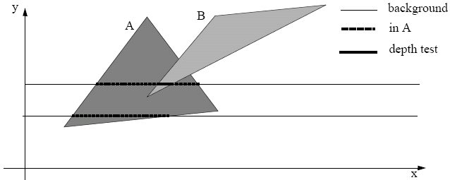
Z-Buffers
The Z (or depth) buffer approach is an image precision approach. We can consider it similar to the frame buffer, which stores colours, as the depth buffer stores Z values. We can manipulate the Z buffer in a number of ways, e.g., we can read and write to it, or make it read only, or link it to the stencil buffer.
In OpenGL, we implement the depth buffer using glutInitDisplayMode(GLUT_DEPTH | ...), and then glEnable(GL_DEPTH_TEST) and then modify glClear() to use the GL_DEPTH_BUFFER_BIT too.
Z-buffering is good as it is not limited to polygons, but any geometric form with depth and colour. Additionally, it has clear memory requirements and it is fairly easy to implement in hardware. The buffer can be saved and reused for further optimisations, and masking can be used to overlay objects.
It does, however, have finite accuracy, and problems can be caused by the non-linear Z transform in perspective projections. Additionally, colinear edges with different starting points can cause aliasing problems to occur, which is why it is important to avoid T-junctions in models.
An improvement that we can use is an A-buffer, which stores a surface list along with RGB intensity, opacity, depth, area, etc... OpenGL only implements a Z-buffer, however, which causes problems as the results of blending can be dependent on the order in which the model objects are rendered. Typically the best way to work round this is to do translucent things last.
Ray Casting
Ray casting works by firing rays from the centre of projection into the scene via the viewplane. The grid squares on the viewplane correspond to pixels, and this way finds the surface at the closest point of intersection, and the pixel is then coloured according to the surface value.
To do this, we need a fast method for computing the intersections of lines with arbritary shapes of polygons. One way of doing this is to represent lines in their parametric form, and then approximate values can be found by subtracting the location of the centre of projection from the pixels position.
This is quite easy for spheres, as using the parametric form of the equation for a sphere gives us a quadratic equation that has two real roots if the line intersects the sphere, a real and complex root if the line is tangential to the sphere and two complex roots if the line does not intersect.
For polygons, the intersection of a line and the plane of a polygon must be found, and then that point must be tested to see if it is inside the polygon.
List Priority
This is a hybrid object/image precision algorithm that operates by depth sorting polygons. The principle is that closer objects obscure more distant objects, so we order the objects to try and ensure a correct image.
The trivial implementation of this is the painters algorithm, which makes the assumption that objects do not overlap in z. In the painters algorithm, you start by rendering the further object away and then draw the closer objects on top - sort, then scan convert. However, if you have overlapping z-coordinates and interpenetrating objects and cyclic overlaps, then problems can occur.
Scan Line Algorithms
In scan line algorithms, these operate by building a data structure consisting of polygon edges crossreferenced to a table of polygons. When a scan commences, all the edges the scanline crosses are placed in an active set. As the scan proceeds, the polygons that it enters are marked as active. If only one polygon is rendered, then its colour is rendered, else a depth test is carried out. This is again an image precision algorithm.
Area Subdivision Algorithms
This is a recursive divide and conquer algorithm. They operate by examining a region of the image plane and applying a simple rule for determining which polygons should be rendered in that region. If the rule works, that area of the polygon is rendered, otherwise, it subdivides and the algorithm is recursively called on each subregion, this continues down to a subpixel level which allows us to sort out aliasing problems. These are mixed or object precision algorithms.
Clipping
Angel c.8.4-8.7The purpose of clipping is to remove objects or parts of objects that lie outside of the view volume. Operationally, the acceleration that occurs in the scan conversion process is sufficient to make this process worthwhile.
If we have a rectangular clip region, then we can consider the basic case of making sure x and y are between the two known bounds of the clip region. Clipping is usually applied to points, lines, polygons, curves and text.
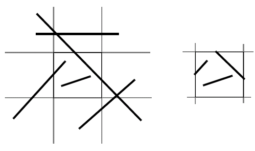
An alternative method with the same effect is scissoring, which is carried out on the pixels in memory after rasterisation, and is usually used to mask part of an image. Clipping, on the other hand, operates with primitives which is discards, creates or modifies. It is more expensive than scissoring, but does greatly speed up rasterisation.
Coden-Sutherland Algorithm
The Cohen-Sutherland algorithm uses the limits of the view volume to divide the world up into regions and assigns codes called "outcodes" to these regions. Line segments can then be classified by the outcodes of their end points. These outcodes are assigned to line midpoints and the outcodes are tested with the results of either accept, reject or split. This is done until all line segments are accepted or rejected.
An outcode consists of 4 bits: (y > ymax)(y < ymax)(x > xmax)(x < xmax), so at any point, the outcode would look like:
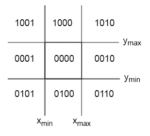
The algorithm works by testing the outcodes at each end of a line segment together with the and of the outcodes. From this, we can infer 4 conditions:
| Outcode 1 | Outcode 2 | Outcode 1 & Outcode 2 | Results |
|---|---|---|---|
| 0 | 0 | Don't care | Both ends in view volume, so render |
| 0 | > 0 | Don't care | One end in and one end out of view volume, clip line to view volume |
| > 0 | 0 | Don't care | |
| > 0 | > 0 | 0 | Part of line may be in view, so do more tests |
| > 0 | > 0 | >0 | Line can not enter view volume |
The Cohen-Sutherland algorithm works best when the clipping region is large compared to the world, so there are lots of trivial accepts, or when the clipping region is small compared to the world, so there are lots of trivial rejects.
However, as we find the intercept using the slope-intercept form, these calculations involve floating point divisions to find x and the value of m, and redundant clipping can often occur.
Parametric Clipping
For equations, see
lecture notes.
This algorithm works by deriving the line equation in a parametric form so the properties of the intersections with the sides of the view volume are qualitatively analysed. Only if absolutely necessary are the intersections carried out.
When we are dealing with 3D, lines have to be clipped against planes. The Cohen-Sutherland algorithm can be applied in a modified form, but only the Ling-Barsky algorithm can be used if parametric clipping is used.
Sutherland-Hodgman
When dealing with polygons, it is not good enough to do line clipping on the polygon edges, as new points must be added to close up polygons. The Sutherland-Hodgman algorithm clips all the lines forming the polygon against each edge of the view volume in turn.
This is implemented conceptually by using in and out vertex lists. The input list is traversed with vertices stored in the output list. Each edge is then clipped against in turn, using the output from the previous clip as input. We can consider this as a pipeline of clippers, and optimise by passing each vertex to the next clipper immediately (i.e., pipelining).
When dealing with curves and circles, we have non-linear equations for intersection tests, so we utilise bounding information for trivial accept/rejects and then repeat on quadrants, octants, etc..., and either test eachs ection analytically or scissor on a pixel-by-pixel basis.
Similarly with text, we can consider it as a collection of lines and curves (GLUT_STROKE) and clip it as a polygon, or as a bitmap (GLUT_BITMAP), which is scissored in the colour buffer. Since characters usually come as a string, we can accelerate clipping by using individual character bounds to identify where to clip the string.
Scan Conversion (Rasterisation)
Angel c.8.9-8.12Given a line defined on the plane of real numbers (x, y) and a discrete model of the plane (x, y) consisting of a rectangular array of rectangles called pixels which can be coloured, we want to map the line on to the pixel array, while satisfying and optimising the constraints of maintaing a constant brightness, having a differing pen style or thickness, the shape of the endpoints if the line is thicker than one pixel and to minimise jagged edges.
The pixel space is a rectangle on the x, y plane bounded by xmax and ymax. Each axis is divided into an integer number of pixels Nx, Ny, therefore the width and height of each pixel is (xmax/Nx, ymax/Ny). Pixels are referred to using integer coordinates that either refer to the location of their lower left hand corners or their centres. Knowing the width and height values allow pixels to be defined, and often we assume that width and height are equal, making the pixels square.
Digital Differential Analyser Algorithm
This algorithm assumes that the gradient satisfies 0 ≤ m ≤ 1 and all other cases are handled by symmetry. If a line segment is to be drawn from (x1, y1) to (x2, y2), we can compute the gradient as m = Δy/Δx. Using a round function to cast floats to integers, we can move along the line and colour pixels in. This looks like:
line_start = round(x1);
line_end = round(x2);
colour_pixel(round(x1), round(y1));
for (i = line_start + 1; i <= line_end; i++) {
y1 = y1 + m;
colour_pixel(i, round(y1));
}
Bresenham's Algorithm
The DDA algorithm needs to carry out floating point additions and rounding for every iteration, which is inefficient. Bresenham's algorithm operates only on integers, requiring that only the start and end points of a line segment are rounded.
If we assume that 0 ≤ m ≤ 1 and (i, j) is the current pixel, then the value of y on the line x = i + 1 must lie between j and j + 1. As the gradient must be in the range of 0 to 45º, the next pixel must either be in the quadrent to the east (i + 1, j) or north east (i + 1, j + 1) (assuming that pixels are identified about their centres).
This gives us a decision problem, so we must find a decision variable to be detected to determine which pixel to colour. We can rewrite the straight line equation as a function ƒ(x, y) = xΔy - yΔx + cΔx. This function has the properties of ƒ(x, y) < 0 when the point is above the line and ƒ(x, y) > 0 when the point is below the line. We can define a line from the centre of our current pixel P to a midpoint of the line between pixels E and NE, that is the point (xP + 1, yP + 0.5).
Following steps are not independent of previous decisions as the line must still extend from the origin of our original pixel P to the midpoint of the E and NE of the current pixel being considered.
To eliminate floats from this, we can simply multiply everything by 2 to eliminate our 0.5 factor.
We have other considerations, such as line intensity. Intensity is a function of slope, and lines with different slopes have different numbers of pixels per unit length. To draw two such lines with the same intensity, we must make the pixel intensity a function of the gradient (or simply use antialiasing).
We can also consider clip rectangles. If a line segment has been clipped at a clipping boundary opposite an integer x value and a real y value, then the pixel at the edge is the same as the one produced by the clipping algorithm. Subsequent pixels may not be the same, however, as the clipped line would have a different slope. The solution to this is to always use the original (not clipped) gradient.
For filled polygons, we calculate a list of edge intersections for each scan line and sort the list in increasing x. For each pair in the list, the span between the two points are filled. When given an intersection at some fractional x value, we determine the side that is the interior by rounding down when inside, and up when outside. When we are dealing with integer values, we say that leftmost pixels of the span are inside, and rightmost are outside. When considering shared vertices, we only consider the minimal y value of an edge, and for horizontal edges, these edges are not counted at all.
We can also use the same scan line algorithm that was discussed in visible surface determination, where a global list of edges is maintained, each with whatever interpolation information is required. This mechanism is called edge tables.
Colours
Colours are used for printing, art and in computer graphics. Colours have a hue, which is used to distinguish between different colours, and this is decided by the dominant wavelength; a saturation (the proportions of dominant wavelength and white light needed to define the colour), which defined by the excitation purity; and a lightness (for reflecting objects) or brightness (for self-luminous objects) called a luminance, which gives us the amount of light.
A colour can be categorised in a function C(λ) that occupies wavelengths from about 350 to 780 nm, and the value for a given wavelength in λ shows the intensity for that colour at that wavelength. However, as the human visual system works with three different types of cones, our brains do not receive the entire distribution across C(λ), but rather three values - the tristimulus values.
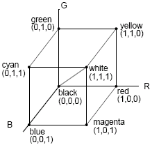
Tristimulus theory is the basic tenet of three-colour theory: "If two colours produce the same tristimulus values, then they are visually indistinguishable". This means that we only need three colours (primaries) to reproduce the tristimulus values needed for a human observer. With CRTs, we vary the intensity of each primary to produce a colour, and this is called additive colour (where the primary colours add together to give the perceived colour). In such a system, the primaries red, green and blue are usually used.
The opposite of additive colour (where primaries add light to an initially black display) is subtractive colour, where we start with a white surface (such as a sheet of paper) and add coloured pigments to remove colour components from a light that is striking the surface. Here, the primaries are usually the complementary colours - cyan, magenta and yellow.
If we normalise RGB and CYM to 1, we can express this as a colour solid, and any colour can therefore be represented as a point inside this cube.
One colour model is the CIE (Commision Internationale de l'Eclairage, 1931). It consists of three primaries: X, Y and Z and experimentally determined colour-matching functions that represents all colours perceived by humans. The XYZ model is an additive model.
The CIE model breaks down colour into two parts, brightness and chromaticity. In the XYZ system, Y is a measure of brightness (or luminance), and the colour is then specified by two derived parameters x and y, which are functions of all tristimulus values, X, Y and Z, such that: x = X/(X + Y + Z) and y = Y/(X + Y + Z).
A colour gamut is a line or polygon on the chromacity diagram
YIQ is a composite signal for TV defined as part of the NTSC standard. It is based on CIE in that the Y value carries the luminance as defined in CIE and I (in-phase) and Q (quadrature) contribute to hue and purity.
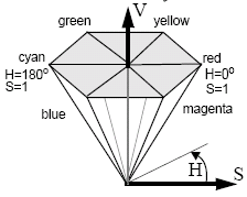
Two other systems are the hue-saturation-value (HSV) system, which is a hexcone represented by the RGB colour space as viewed from (1, 1, 1) and is represented as an angle around the cone (hue), the saturation (distance from the origin) as a ratio of 0 to 1 and value (intensity), which is the distance up the cone.
A similar system is the hue-lightness-saturation (HLS) system. The hue is the name of the colour, brightness the luminance and saturation the colour attribute that distinguises a pure shade of a colour from a shade of the same hue mixed with white to form a pastel colour. HLS is also typically defined as a cone, so it represents and easy way to convert the RGB colour space into polar coordinates.
Illumination
Angel c.6
The simplest lighting model is that where each object is self-luminous and has its own constant intensity. This is obviously not very accurate, however, so we consider light to originate from a source, which can either be ambient, a spotlight, distributed or a distant light.
Surfaces, depending on their properties (e.g., matte, shiny, transparent, etc) will then show up in different ways depending on how the light falls on. We can characterise reflections as either specular, where the reflected light is scattered in a narrow range of angles around the angle of reflection, or as diffusing, where reflected light is scattered in all directions. We can also consider translucent surfaces, where some light penetrates the surface using refraction, and some is reflected.
Diffuse Reflection
We can use the Lambertian model to implement diffuse reflection, which occurs on dull or flat surfaces.
With the Lambertian model, the light is reflected with an equal intensity in all directions (this is not a real world representation, however, as imperfections in a surface will reflect light more in some directions than others), however we only consider the vertical component of the light (the angle between the surface normal N and the light source L, which can be represented as ( ∧ ). We also need to consider a diffuse reflection coefficient k, so we can compute the intensity of a surface as I = Isourcek( ∧ ).
We can also consider a distance term to account for any attenuation of the light as it travels from the source to the surface. In this case, we use the quadratic attenuation term k/(a + bd + cd2), where d is the distance from the light source.
However, this causes problems as the value will be negative if it is below the horizon, so we give this value a floor of 0.
For long distance light sources, we can consider to be constant, and harshness can be alleviated by including an ambient term.
Diffuse reflection is set up using GL_DIFFUSE or GL_AMBIENT_AND_DIFFUSE in glMaterial.
Specular Reflection
Specular reflection is a property of shiny (smooth) surfaces. If we assume point sources, we can have a model as follows:
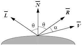
Where is the light source vector, is the surface normal and is a vector towards the centre of projection. In a perfect reflector, reflections are only along .
Phong Illumination
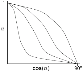
The Phong illumination model is a simple model for non-perfect reflectors. Maximum reflection occurs when α is 0, and then a rapid fall-off occurs. It can be approximated by cosn(α), where n is a shininess coefficient.
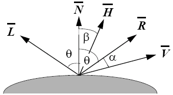
The Phong illumination model including distance attenuation is therefore: I = Isourceksource + ((kcosθ + kspecularcosnα)Iambient)/(a + bd + cd2), where we now have a new specular-reflection coefficient, kspecular.
For multiple light sources, lighting equations are evaluated individually for each source and the results are summed (it is important to be aware of overflow).
Objects that appear further from the light appear a darker. A realistic but unhelpful way of modelling this is as 1/(d2), so we use the more useful model min(1/(a + bd + cd2), 1), where a, b and c are constants chosen to soften the lighting.
In OpenGL, we can use the parameters GL_CONSTANT_ATTENUATION, GL_LINEAR_ATTENUATION and GL_QUADRATIC_ATTENUATION to allow each factor to be set.
Fog
Atmospheric attenuation is used to simulate the effect of atmosphere on colour, and is a refinement of depth cueing. It is most commonly implemented using fog.
OpenGL supports three fog models using glFog{if}v(GLenum pname, TYPE *params);, which using the GL_FOG_MODE parameter with the arguments GL_LINEAR, GL_EXP or GL_EXP2. Other parameters for glFog include GL_FOG_START, GL_FOG_END and GL_FOG_COLOR.
Additionally, fog must be specifically enabled using glEnable(GL_FOG);.
Global Illumination
Global illumination takes into account all the illumination which arrives at a point, including light which has been reflected or refracted by other objects. It is an important factor to consider when persuing photo realism.
The two main global illumination models are ray tracing, which considers specular interaction, and radiosity, which considers diffuse interaction. When considering these with regard to global illumination, we have global interaction, where we start with the light source and follow every light path (ray of light) as it travels through the environment. Stopping conditions that we can consider are when the light hits the eye point, if it travels out of the environment, or if the light has had its energy reduced to an admisible limit due to absorbtion in objects.
With diffuse and specular interactions, we can derive four types of interaction to consider, diffuse-diffuse (the radiosity model), specular-diffuse, diffuse-specular and specular-specular (ray tracing).
Ray Tracing
Whitted ray tracing is a ray tracing algorithm that traces light rays in reverse direction of propagation from the eye back into the scene towards the light source. Reflection rays (if reflective) and refraction rays (if translucent/transparent) are spawned for every hit point (recursive calculation), and these rays themselves may spawn new rays if there are objects in the way.
Ray tracing uses the specular global illumination model and a local model, so it considers diffuse-reflection interactions, but not diffuse-diffuse.
The easiest way to represent ray tracing is using a ray tree, where each hit point generates a secondary ray towards the point source, as well as the reflection and refraction rays. The tree gets terminated when secondary rays miss all objects, a preset depth limit is reached, or time/space/patience is exhausted.
Problems with ray tracing are that shadow rays are usually not refracted, and problems with numerical precision may give false shadows. Additionally, the ambient light model it uses is simplistic.
Radiosity
Classic radiosity implements a diffuse-diffuse interaction. The solution is view-independent, as lighting is calculated for every point in the scene, rather than those that can be seen from the eye.
With radiosity, we consider the light source as an array of emitting patches. The scene is then split in to patches, however this depends on the solution, as we do not know how to divide the scene in to patches until we have a partial result, which makes the radiosity algorithm iterative. We then shoot light in the scene from a source and consider diffuse-diffuse interactions between a light patch and all the receiving patches that are visible from the light patch. The process then continues iteratively by considering as the next shooting patch the one which has received the highest amount of energy. The process stops when a high percentage of the intial light is distributed about the scene.
Problems can occur if the discretisation of the patches is too course, and radiosity does not consider any specular components.
Shading
Angel c.6.5 There are two principle ways of shading polygons, using flat shading, where 1 colour is decided for the whole polygon and all pixels on the polygon are set to that colour, or interpolation shading, where the colour at each pixel is decided by interpolating properties of the polygons vertices. Two types of interpolation shading are used, Gourand shading and Phong shading. In both Gourand and Phong shading, each vertex can be given different colour properties and different surface normals.
Flat Shading
In this model, the illumination model is applied once per polygon, and the surface normal N is constant for the entire polygon - so the entire polygon is shaded with a single value.
This can yield nasty effects (even at high levels of detail), such as mach banding, which is caused by "lateral inhibition", which is a perception property of the human eye - the more light a receptor receives the more it inhibits its neighbours. This is a biological edge detector, and the human eye prefers smoother shading techniques.
In OpenGL, this model can be used using glShadeModel(GL_FLAT).
Gourand Shading
In Gourand shading, each vertex has a normal vector and colour data associated with it. The colouring of each vertex is then determined and then interpolated along each edge. When the polygon is then scan converted, the colour is interpolated along each scan line using the edge values.
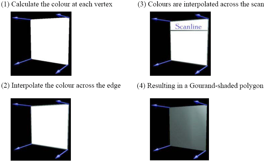
However, the polygons are still flat, so the silhouette of curved objects can visibly consist of straight lines. Additionally, in the OpenGL pipeline, shading is carried out after the projection transformation is applied, so if a perspective transformation is used, the non-linear transformation of the Z-axis may produce odd effects. These effects can be worked around using smaller polygons, however.
Additionally, discontinuities can occur where 2 polygons with different normals share the same vertex, and odd effects can occur if the normals are set up wrong, and some mach banding effects can still be produced.
In OpenGL, this mode is used using glShadeModel(GL_SMOOTH).
Phong Shading
In Phong shading, the normals are interpolated rather than the colour intensities. Normals are interpolated along edges, and then interpolation down the scan line occurs and the normal is calculated for each pixel. Finally, the colour intensity for each pixel is calculated.
Phong shading does give a correct specular highlight and reduces problems of Mach banding, but it does have a very large computational cost, so Phong shading is almost always done offline, and it is not available in standard OpenGL.
Blending
We can use a process called blending to allow translucent primitives to be drawn. We consider a fourth colour value - the alpha value (α ∈ [0,1]) - to give us a RGBA colour model. Alpha is then used to combine colours of the source and destination components. Blending factors (four-dimensional vectors) are used to figure out how to mix these RGBA values when rendering an image. A factor is multiplied against against the appropriate colour.
In OpenGL, blending must be enabled using glEnable(GL_BLEND) and the blending functions for the source and destination must be specified using glBlendFunc(GLenum source, GLenum destination). Common blending factors include:
| Constant | Blending Factor |
|---|---|
| GL_ZERO | (0, 0, 0, 0) |
| GL_ONE | (1, 1, 1, 1) |
| GL_SRC_COLOR | (Rsource, Gsource, Bsource, Asource) |
| GL_ONE_MINUS_SRC_COLOR | (1 - Rsource, 1 - Gsource, 1 - Bsource, 1 - Asource) |
| GL_SRC_ALPHA | (Asource, Asource, Asource, Asource) |
| GL_ONE_MINUS_SRC_ALPHA | (1 - Asource, 1 - Asource, 1 - Asource, 1 - Asource) |
The order in which polygons are rendered affects the blending.
Shadows
There are two methods to implement shadows:
- Use solid modelling techniques to determine shadow volumes, then change the scan conversion routine to check if a pixel is in a shadow volume, and reduce slightly the colour intensity for every volume they are in.
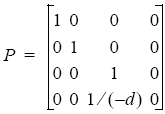
- A cheaper way is to consider only shadows on one plane then define a perspective projection onto that plane with the centre of projection being the light source. To do this, we first draw the plane, then any other objects and multiply the view matrix by the perspective projection matrix, switch the depth testing and re-render the objects. This is also called 2-pass shading, and uses the following simple projection matrix that projects all 3D points onto a 2D plane a distance d from the centre of projection.
Texturing
Angel c.7.6To provide surface detail, geometric modelling has its limits - a large number of polygons are inefficient to render and there is a modelling problem to implement them. It is often easier to introduce detail in the colour/frame buffer as part of the shading process. Tables and buffers can be used to alter the appearance of the object, and several different mapping approaches are in widespread use, e.g., texture mapping is used to determine colour, environment mapping to reflect the environment and bump mapping to distort the apparent shape by varying the normals.
A texture is a digital image that has to be mapped onto the surface of the polygon as it is rendered into the colour buffer. Many issues can arise during this process, such as differences in format between the colour buffer and the image, the number of dimensions in the texture, the way the image is held (should be as a bitmap consisting of texels), and how the image is mapped to the polygon.
Texture Mapping
Translating textures in multiple dimensions to a 2 dimensional polygon can be done in a number of ways:
- 1-dimensional, e.g., a rainbow - a 1-dimensional texture from violet to red is mapped onto an arc
- 2-dimensional - this is straight forward as a direct mapping can be done
- 3-dimensional, e.g., a sculpture, a 2-dimensional texture contains a 3-dimensional model of the rocks colouring and a one-to-one mapping of the space containing the statue onto the texture space occurs. When the polygons of the statue are rendered, each pixel is coloured using the texture colour at the equivalent texture space point
- 4-dimensional - a 3-dimensional mapping is done, and the fourth dimension should consist of the initial and last states and the intermediate steps are the alpha blends of the two limits. Consecutive textures are then applied during the animation.
When we have a two-dimensional texture consisting of a 2-dimensional array of texels and a 2-dimensional polygon defined in 3-dimensional space and then a mapping of the texture on to the polygon, we can project the polygon onto a viewplane then quantise the viewplane in to discrete pixels. We then need to use the correct texel for any pixel on the polygon. OpenGL explicitly supports 1-dimensional and 2-dimensional textures.
One way of doing this is to normalise the texture space (s, t) to [0,1] and then consider the mapping of a rectange of texture in to the model (u, v) space. This mapping is defined parametrically in terms of maximum and minimum coordinates - u = umin + (s - smin)/(smax - smin) × (umax - umin).
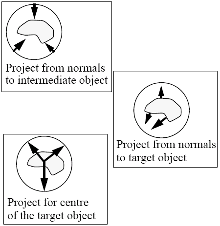
An alternative is to texture a whole object at once using a projection from a simpler intermediate object - this process is called two-part mapping. Textures are mapped on to regular surfaces (e.g., spheres, cylinders, boxes) and projected on to the textured object using three different methods - the normal from the intermediate, the normal to the intermediate and the projector from the centre of the object. All that then has to be done is to define the mapping on to the intermediate object.
If there is more polygon than there is texture, we can either repeat the whole texture like wall paper, or repeat only the last bits of the texture as a 1-dimensional texture. Additionally, sampling problems between the texture and the polygon can occur, which is further heightened by the non-linear transformation of the Z-axis in the case of perspective. Mipmapping can be used to control the level of detail by generating new textures that have half the resolution of the original and using them where appropriate.
In OpenGL, textures are defined as a combination of an image bitmap and a mapping function on to objects. The image bitmap is set using glTexImage2D(GLenum target, GLint level, GLint components, GLsizei width, GLsizei height, GLint border, GLenum format, GLenum type, GLvoid *pixels). Where target is normally either GL_TEXTURE_2D or GL_TEXTURE_1D (a glTexImage1D() variant also exists), level is normally 0 and allows multi-resolution textures (mipmaps), components are the number of colour components (1-4, i.e., RGBA), width and height are the horizontal and vertical dimensions of the texture map and need to be a power of 2, border is either 0 or 1 and defines whether or not a border should be used, format is the colour format (e.g., GL_RGB or GL_COLOR_INDEX), type is the data type (e.g., GL_FLOAT, GL_UNSIGNED_BYTE) and pixels is a pointer to the texture data array.
glTexParameter{if}v(GLenum target, GLenum parameter, TYPE *value), is used to determine how the texture is applied. target is typically GL_TEXTURE_2D and parameter is one of GL_TEXTURE_WRAP_S, GL_TEXTURE_WRAP_T, GL_TEXTURE_MAG_FILTER, GL_TEXTURE_MIN_FILTER and GL_TEXTURE_BORDER_COLOR. The value then depends on the parameter being set. The wrap parameters determine how texture coordinates outside the range 0 to 1 are handled and the values GL_CLAMP is where the coordinates are clamped to the range 0..1 so the final edge texels are repeated and GL_REPEAT repeats the whole texture along the fractional parts of the surface. MAG and MIN specify how texels are selected when pixels do not map on to texel centres. GL_NEAREST is used to select the nearest pixel and GL_LINEAR uses a weighted average of the 4 nearest texels. GL_TEXTURE_BORDER_COLOR expects a colour vector to be specified as a parameter.
The vertices of the polygon must be assigned coordinates in the texture space and this is done in the same way as assigning normals, with a glTexCoord2f(x, y) command, which assigns the vertex to position (x, y) in the 2-dimensional texture.
glTexEnvi(GL_TEXTURE_ENV, GL_TEXTURE_ENV_MODE, value) is used to determine the interaction between texture's and the polygon's materials, where value is either GL_REPLACE, where the pixel is always given the texture's colour; GL_DECAL, where in RGB the pixel is given the texture's colour, but if RGBA is used, alpha blending occurs; GL_MODULATE is where the polygons colour and texture are multiplied; and GL_BLEND where a texture environment colour is specified using glTexEnvfv(GL_TEXTURE_ENV, GL_TEXTURE_ENV_COLOR, GLfloat *colourarray) and this is multiplied by the texture's colour and added to a one-minus texture blend.
As with most other things in OpenGL, we also need to use glEnable(GL_TEXTURE_2D) and glEnable(GL_TEXTURE_1D) to enable texturing.
Mipmapping
Mipmapping is implemented in OpenGL where the resolution of a texture is succesively quartered (e.g., 1024 × 512 → 512 × 256 → 256 × 128 → ... → 1 × 1 ).
OpenGL allows different texture images to be provided for multiple levels, but all sizes of the texture, from 1 × 1 to the max size, in increasing powers of 2 must be provided. Each texture is identified by the level parameter in glTexImage?D, and level 0 is always the original texture. The use of it is activated by glTexParameter() with the GL_TEXTURE_MIN_FILTER and the GL_NEAREST_MIPMAP_NEAREST parameters.
OpenGL does provide a function to automatically construct mipmaps: glBuild2DMipmaps(GLenum target, GLint comps, GLint width, GLint height, GLint format, GLenum type, GLvoid *data). All the parameters are the same as they are in glTexImage().
Texture Blending and Lighting
Additionally, we need to consider blending and lighting the texture. When a texel is to be placed in to the colour buffer during scan conversion, we still need to make two choices - whether or not the illumination model applies to the texture and whether the texture replaces the properties of the underlying material of the polygon, or be blended with it (i.e., do we only see the texture, or a mixture of texture and material). If we do not apply the illumination model to the texture, the texture will appear the same from all angles under all lights, and if we do then the texture will be shaded using the same calculations as would be applied to material properties of the polygon.
Enviroment and reflection maps can be used to simulate a shiny object without ray tracing. A view point is positioned within the object, looking out and then the resultant image is used as a texture to apply to the object. The reflective object S is replaced by a projection surface P and then the image of the environment is computed on P. An image is then projected from P onto S.
Many other pixel-level operations are also possible:
- Fog - the pixels are blended with the fog colour with the blending governed by the Z-coordinate
- Antialising - pixels are replaced by the average of their own and their nearest neighbours colours
- Colour balancing - colours are modified as they are written in to the colour buffer
- Direct manipulation - colours are copied or replaced
As well as the colour and depth buffers, OpenGL provides a stencil buffer used for masking areas of other buffers, an accumulation buffer which can be used for whatever you want and a bitwise XOR operator is usually provided in hardware on the graphics chip.
Halftones
Halftones can be used to increase apparent available intensities at the expense of resolution and are based on the principle of halftoning as used in newspaper and other print publications.
Halftones are implemented using rectangular pixel regions called halftone patterns. An n2 grid gives n2 + 1 intensities, so a 4 by 4 block has 17 shades from white to black. To reach a level k intensity, you need to turn on the pixels numbered ≤ k. This can be generalised to colour.
Pattern generation is not trivial, as sub-grid patterns become evident. Visual effects, e.g., contouring, need to be avoided, and isolated pixels are not always effective on some devices.
Dithering
Dithering uses the same principle as halftone in printing, but the output medium has fixed pixels and can not represent the dots of a half tone picture. The solution is to use a block of pixels for each point in the image.
For an n × n dither matrix Dn, entries are 0..n2 - 1. The input intensity IR required at (x, y) is scaled in to 0 ≤ k ≤ n2. (x, y) is then only turned on if and only if IR > ID.
If the number of pixels in the colour buffer is the same as in the output medium, dithering is applied by incrementing the intensity of each pixel in the output by components dependent on the sum of the values from several superimposed dither matrices representing the pixels of the input.
Dithering in OpenGL can be implemented using glEnable(GL_DITHER) and glDisable(GL_DITHER), but by default it is enabled.
Bump Maps
Bump maps are used to capture surface roughness. A pertubation function is applied to the surface normal and this pertubed normal is used in lighting calculations. At a position in the surface P(u, v) and a bump map b(u, v), then the surface effect P′(u, v) = P(u, v) + b(u, v)n.
Bump maps are represented using lookup tables and can be random patterns, regular patterns or some other mapping, such as characters, etc...
OpenGL provides facilities for all or part of a texture image to be replaced by a new image with glTexSubImage2D(), as it is much faster to replace than to construct a new image - this is useful in video processing. Additionally, glCopyTexImage?D() and glCopyTexSubImage?D() allow you to take texture information directly from the frame buffer.
OpenGL implementations may support working sets of textures called texture objects, which are similar in principle to display lists. With these, you can enquire the state of textures and available resources, prioritise textures and release texture resources with glDeleteTextures(). glTexGen() can be used for the automatic generation of texture coordinates allowing sphere and cube mappings. Additionally, a texture matrix exists which can transform the texture coordinates. This is used with animation to produce moving (4-dimensional) textures.
Visualisation
Visualisation is the process of generating graphical models from data. Many computer based technologies generate massive amounts of data, such as satellite and spacecraft scanners, medical instruments (CT, MRI, ultrasound, etc), simulations of fluid dynamics and weather forecasting, financial data and information spaces. Automated analysis is of limited use when trying to make sense of very large datasets, so it makes sense to utilise human visual capabilities - IA, rather than AI. The challenge is therefore to extract a graphical model from the data.
Visualisation is a somewhat biased term, as we can "visualise" things using our auditory senses (sonification) and based on physics (haptics), so we can say that our ultimate aim is conceptualisation. With visualisation, we can also have collaborative visualisation and computational steering, where the computer attempts to apply some analysis to the data to help the user.
We can break down the visualisation process into two areas, the system and the user. The system takes data, applies it to a model and then renders the result. The user takes this result and perceives it, applying structure and eventually understanding it.
Two main types of visualisation are scientific visualisation and information visualisation. If the data has a natural mapping to R3, then we can use scientific visualisation, otherwise information visualisation has to be used.
Visualisation Pipeline
Most visualisation systems consist of a pipeline of processes, and some powerful commercial tools implement these in a visual programming environment, where visualisation modules are plugged together by data flows. The system can then automate updates of results when the parameters or models change.
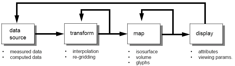
Scientific Data Sets
We can classify scientific data sets on four orthogonal criteria:
- Dimensionality
- Attribute data type (scalar, vector, tensor, multivariable, etc)
- Cell type (vertex, triangle, etc)
- Organisation of cells (topological and geometrical)
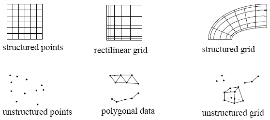
Some examples of visualisation include contour data, which can be shown as a 3 dimensional mesh, or a 2-dimensional grid, with colour representing the third dimension. Voxels can also be used when representing 3-dimensional data, such as that from an MRI scanner. Here, the source data consists of parallel planes of intensity information collective from consecutive cross sections - in MRI a pixel of such a plane represents the X-ray absorption of that part of the body that the pixel physically corresponds to, so corresponding pixels in two consecutive planes form the top and bottom of a voxel.
Vector fields and flows can also be represented using a directed line segment, where length is proportional to magnitude. Care is required for scaling and foreshortening, and the data also needs to be filtered to reduce clutter. Variations of this exist, such as using glyphs.
Flow visualisation (such as in wind tunnels and ultrasound) and be represented using a particle track, which traces the path of a particle in the field. Streamlining allows you to integrate the flow over time.
Optical flow and motions can be represented using pindiagrams (arrows) showing the direction of the displacement.
On the other hand, data sets for information visualisation are more disparate, and are either of implicit functions (i.e., ƒ(x, y) = c) or explicit functions (i.e., z = g(x, y)).