CGO builds upon the knowledge previously taught in LSA, which focussed on the front end (lexing and parsing) of compiler construction.
Compiler Passes
A good compiler has various requirements, including:
- correctly implementing the language;
- detecting all static errors;
- user interface: precise and clear diagnostics and easy to use processing options;
- generating optimised code;
- compiling quickly using modest resources;
- structure: modular, with low coupling, well-documented and maintainable with lots of internal consistency checking.
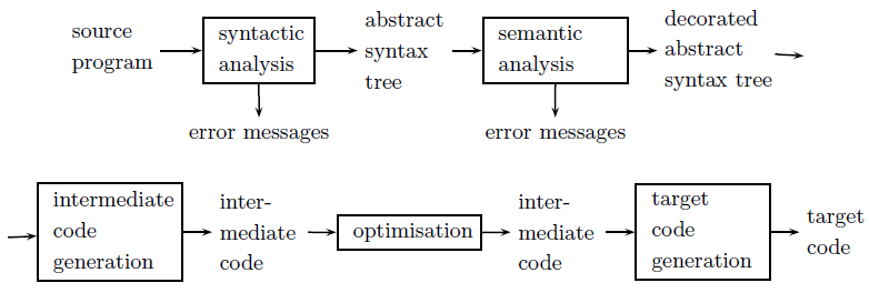
The pipeline represents the various stages, from a front end dealing with the source language (analysis), to a backend in the target language (synthesis). A properly modular architecture allows for reuse of the backend components between different frontend languages.
A pass is a traversal of a program or its representation. In a multi-pass setup, the compiler driver drives the syntactic analyser, semantic analyser and code generator separately (i.e., each one passes over the code). This gives us modularity, advanced optimisations and more freedom for the source language.
In a single pass setup, the compiler driver only drives the syntactic analyser, which in turn triggers the semantic analyser and code generator. This means code is partially generated as the code is parsed, and therefore only one pass is required. This gives us a compiler that is faster and uses less space, but some obscure language constructs may require information from the semantic analyser in the syntactic analyser (e.g., (A)-1 in C), which a single-pass can not cope with.
Semantic Analysis
Static semantics are program constraints - checkable at compile time (as opposed to run time), but are not expressible by a context-free grammar. These constraints include elements such as:
- scope rules, which govern occurences of identifiers in declarations and in use;
- type rules, which determine the type of expressions, and whether a program is well-typed;
- name-related checks;
- flow-of-control checks;
- apply precedence and associativity of user-defined operators, etc
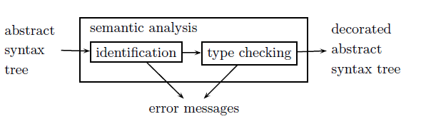
The semantic analysis phase checks static semantics and augments the abstract syntax tree (e.g., with type information, etc). The main subphases of this phase are identification, checking the scope rules and connecting all occurrences of an identifier within the same scope, and type checking - inferring types and checking type rules, and possibly augments expressions with their types.
Identification
A declaration binds an identifier to some meaning.
A scope is a region of program delimited by program constructs (e.g., { ... }). The scope of a declaration is the region of the program in which the declaration is active.
Modern languages have similar scope rules, these are the most common:
- Every use of an identifier must be in the scope of a definition of the identifier.
- An identifier may only be declared once per scope.
- Scopes may be nested.
- The scope of a declaration is the scope in which it appears, plus every nested scope inside that scope where it has not been hidden.
- A declaration hides a declaration of the same identifier in its scope and internally nested scope.
In other words, the declaration of a used identifier is in the smallest enclosing scope that contains a declaration of the identifier.
Identifier have attributes which contain information about a programming language construct. For a variable identifier, this might be type and memory address, or for a function identifier, this might be types of arguments and results, and memory address, etc...
The identification phase connects the identifiers occuring in the abstract syntax tree to a record of attributes (which is filled in by other phases) and reports violation of scope rules. The identifier in a declaration and all occurrences of the identifier in the sope of the declaration share a record.
Symbol Tables
The symbol table is a dictionary data structure mapping identifiers to attribute records.
The identification phases traverses the abstract syntax tree and for each identifier in a declaration, a new attribute record is inserted into the symbol table. When each identifier is used, it is looked up in the symbol table and connected to the found attribute record.
The symbol table is a stack of tables, with a table for each nested scope. Insertion is always in the table for the the innermost scope, and lookup starts first with the innermost scope, moving on to the next enclosing scope if it's not found. Opening and closing a scope is simply putting a new empty table on the stack, or removing the top table from it.
For sequential declaration structure (as in C), the scope of the declaration starts at the beginning of the declaration, and identification can be done in a single program traversal. For mutually recursive declarations (e.g., an f(x) which calls g(x) which can in turn call f(x)), a forward declaration is needed. The scope of declaration starts already at is forward declaration, and identification has to check the consistency of the forward declaration.
For languages such as Java which support recursive declaration structures, the scope of declaration encompasses the whole scope. Identification first inserts all declarations of a scope in the symbol table, and then traverses the scope for lookup of use occurrences. This has the downside of being incompatible with single-pass compilation.
The efficiency of the symbol table has a major impact on the efficiency of the whole compiler, especially lookup.
Standard data structures for a table include a hash table with external chaining (fixed size table with a linked list as buckets), a balanced tree (e.g., red-black tree, 2-3-4 tree or an AVL tree), or a trie (which is good for looking up strings, however a scanner may have replaced identifier strings by a number referring to an identifier table to save space).
Optimisation for a stack of tables also needs to be considered - after lookup, a copy is made of the table in the current scope.
An alternative solution to using one stack of tables is to use one table of stacks. The nesting level is stored as one attribute, opening a scope increases the nesting level, and closing the scope decreases the nesting level and removes all stack entries of a higher level.
With this method, lookup is only needed to be done in one table instead of several (but usually not many nested scopes), and as we never know the right size for a hash table, here one big table is only a minor waste of space. However, closing the scope is less efficient and more complex - making it harder to support the additional features we will discuss later.
In related literature, different approaches to identification may be found, including one where identifiers in the abstract syntax tree are not connected to their attribute record, and the symbol table is passed to subsequent compiler phases.
The disadvantages of this approach include inefficiency - every time an attribute is read or written, the attribute record is searched anew in the symbol table; and complexity - the symbol table has to associate identifiers for all scopes within attributes (either a tree, instead of a stack of tables, or a single table with a serial number per scope and during traversal, a scope stack of serial numbers).
Name Spaces
An identifier may be used for different purposes, even if in the same scope, if uses are in different name spaces. Identifiers in different name spaces, but with the same scope rules, may be stored in the same symbol table with its name space class.
Members/methods are in scope in certain expressions (e.g., myQueue.enqueue(...)). One way to implement this is to have a table of members/methods for every structure/union/class, and this table is linked to from the type entry in the main symbol table. To support inheritance, a list of tree of tables is needed. Often, we need to combine identification with type checking. Furthermore, scope depends on the context (e.g., public, protected, private, etc).
Modules export sets of identifiers, and code and modules can import identifiers from other modules. The simplest symbol table implementation to support this is having a separate table for each export interface, and then connect the tables according to scope rules.
Overloading further complicates matters, as an identifier may have several meanings, depending on the types being used. The symbol table entry must contain attribute records for all the meanings that are in scope. This type information must be in function attributes during identification.
Dynamic Scoping
So far we have covered static (or lexical) scoping. The scope of declaration is determined by the program structure. Dyanamic scoping exists where the scope of the declaration is determined by the control flow (i.e., the current declaration is the last declaration encountered during execution that is still active).
Dynamic scoping is sometimes useful (implicit arguments), but identification and type checking are deferred to run time, and it possibly makes programs harder to understand. Various "safe" variants of dynamic scoping have been deployed.
Type Checking
Type checking is the phase that infers type and checks type rules, possibly augmenting expressions with their types.
Types
Types are sets of values, and values of different types may be represented by the same bits, so we need to know the type in order to interpret a bit pattern.
Type systems exist to prevent occurrence of errors at run time. If an execution error, its effects depend on the implementation details that are not specified by the language (e.g., illegal instruction fault, illegal memory access fault, data corruption). We say an error is untrapped if it goes unnoticed for a while at run time (e.g., writing data past the end of an array in C).
A strong type system guarantees that a specified set of errors can not occur, and this set should include all untrapped execution errors.
Static type systems have type expressions as part of the language systems, and the rules define well-typed programs. It can be checked at compile time if a program is well typed. Some run time checks can still be required if the type system is strong (e.g., array subscripting, subrange types, etc).
Dyanamic typing systems are when the values carry type information at run time, and all type checks are performed at run time.
Static type systems enable generation of better code, as memory requirements of all variables are known, more specific code can be generated, run-time tests can be avoided and less space is needed for run type information. Many errors (including logical ones) can be found at compile time.
Types can be used to describe interfaces of modules, supporting modular software deployment, and independent compilation of modules. Static type systems can guide the design of powerful, but less complex, programming languages. Orthogonal type systems lead to orthogonal languages.
A type is denoted by a type expression. A type expression is:
- a basic type (e.g., int, char, void);
- an application of a type constructor to type expressions (e.g., array, record/structure, class, union, point, function);
- an identifier of a user defined type; or
- a type variable (see parametric polymorphism).
Often type systems are not orthogonal (there is no function as a function argument or result).
a language is polymorphic is it allows language constructs to have more than one type (the opposite being monomorphic). Some languages allow program constructs to be parameterised by type variables - parametric polymorphism.
A type annotation is a restricted form of formal specification. A type system should be decidably verifiable to enforce it. An algorithm ensures that a program meets the properties specified by its types, and some properties are checked at run time. A type system should be transparent. A programmer should be able to predict if a program will type check. Type error messages should be comprehensible.
Basic Type Checking
Basic type checking involves a single traversal of the abstract syntax tree. Only expression have types - declarations and statements do not.
To type check a declaration, the type attribute is filled in for a the declared identifier and the components recursively type checked.
For a statement, the components are recursively type checked, meaning that the type of the expression components meet type rules (e.g., id = exp, id and exp must have equivalent types).
To type check an expression, the type is inferred from the bottom-up, i.e., recursively type check subexpressions and check that types of subexpressions meet type rules. The type rule and types of subexpressions determine the type of the expression.
Type Equivalence
Two types are structually equivalent iff they are the same basic type, or they are applications of the same type constructor to structually equivalent types. A problem is that type systems shall enforce properties of the implemented systems. Often types with the same internal structure shall be distinct.
New types can be declared in Ada as type Celsius is new Float which declares a new type Celsius as distinct from all other types, including Float.
Synonyms can also be declared, e.g., in Ada as subtype Celsius is Float and in C as typedef float Celsius.
The following types in C are distinct, despite being structurally equivalent: struct Celsius { float temp; } and struct Fahrenheit { float temp; }.
Most languages use a mixture of structural and name equivalence, and in some languages, distinct occurrences of type expressions create unique types. Many languages do not define type equivalence precisely.
A type may appear in the type expression that defines it. C permits recursion only in form of pointer to tagged structure or union, similarly other languages use type constructs that are not compared structurally to prevent infinite comparison.
Actually, structurally comparing cycling type expressions is easy. In recursive comparison, assume that all previously visited type pairs are equivalent (equivalence is the largest relation defined by structural equivalence).
Type conversion can be done when types are inequivalent and rules specify which type may be converted into which other type, and how. This is implicit and is done by the type checker.
The two types of conversion are coercion, which usually require a transformation of representation (e.g., int to float), and subtyping, which usually has no representation transformation (e.g., downcasting).
Explicit type conversion can also be done (e.g., in C (float)3).
Overloading
A function identifier is overloaded if in one scope it refers to more than one function. Equality and arithmetic operations are often overloaded. Some languages allow user-defined overloaded functions.
Resolution can be local (as in C), where only the types of the arguments determines which function is meant, or global (as in Ada), when the full usage context is taken into consideration. A program is well typed in global resolution if the types of all subexpressions are unique. Type checking can be one bottom-up and one top-down traversal.
Another form of resolution is at runtime (as in Haskell). The compiler infers predicates over types, and solves constraints to ensure predicates are compatible, perhaps simplifying or eliminating them. At runtime, functions receive dictionaries representing the evidence that a predicate holds.
Attribute Grammars
So far, transformation of an abstract syntax tree (identification, type checking, etc) has been described by an explicit traversal of the tree. However, we can use attribute grammars to define a shorter, implemenation-indpendendent specification.
Transformation is a determination of attributes - an attribute contains information about a programming language construct (e.g., the current symbol table, or even a new tree of intermediate code). If we specifiy attributes locally for each grammar rule, we get syntax direct definition.
Part of an example attribute grammar for an expression type may be:
exp0 → exp1 < exp2
exp0.type = if exp1.type = Int and exp2.type = Int then Bool else error
exp0 → exp1 + exp2
exp0.type = if exp1.type = Int and exp2.type = Int then Int else error
exp → num
exp.type = Int
X.a denotes the attribute a associated with the grammar symbol X. Subscripts denote multiple occurrences of the same symbol. In these particular examples, error may be a special type, or the grammar is intended to be refined later. One thing to bear in mind is that these are expressions, not statements.
Given a context free grammar, we can now define an attribute grammar:
- associates with each grammar symbol X a set of attributes Att(X);
- contains for each grammar rule X0 → X1 ... Xn a set of attribute equations of the form: X.a = exp { Y.b | Y ∈ { X0, ..., Xn }, b ∈ Att(Y) }, where X ∈ { X0, ..., Xn }, a ∈ Att(X) and exp is an expression is some meta-language and may use the listed attributes.
The attribution of a parse tree maps the attributes of all tree nodes to values such that the attribute equations are fulfilled. (Note, attribution actually works on the AST as a representation of the parse tree, but parse tree has a closer relationship to the grammar).
The dependency graph of an attribute equation X.a = exp has a node for each attribute Y.b appearing in the equation and an edge from each node Y.b appearing in the right hand side of the equation to the node X.a on the left-hand side of the equation. An example dependency graph can be superimposed over a parse tree segment corresponding to the grammar rule:
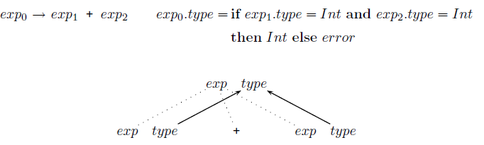
The dependency graph of a grammar rule is the union of the dependency graphs of all the attribute equations associated with the grammar rule.
The dependency graph of a grammar rule is the union of the dependency graphs of all attribute equations associated with the grammar rules analogously to the construction of the parse tree.
An attribution of a parse tree is well-defined if for every attribute a of every tree node X there is one defining attribute equation X.a = exp (actually, there may be no equations for some attributes, because their values are already known from syntax analysis, e.g., Num.value = 6), and the dependency graph of the parse tree is acyclic.
We say a grammar is non-circular if the dependency graph of every parse tree is acyclic. An exponential time decision algorithm for non-circularity exists.
One way to ensure an attribute grammar is well-defined is to ensure that for all attributes X.a, all defining equations X.a = exp either belong solely to productions X → Y1 ... Yn, or belong solely to productions Y0 → Y1 ... X ... Yn, otherwise there will be two conflicting equations for some tree node.
Attribute values can be computed in the order indicated by the dependency graph. In a lazy functional programming language, attribute values can be computed by a single tree traversal. For easy implementation in other languages, further restrictions are needed.
We say an attribute X.a is synthesised if every attribute equation of the form X0.a = exp belongs to a grammar rule X0 → X1 ... Xn and exp contains only attributes of X1, ..., Xn, otherwise an attribute is inherited.
In a parse tree, all dependencies for a synthesised attribute point from child to parent, and all dependencies for an inherited attribute from point parent of sibling to child.
If an attribute grammar consists only of synthesised attributes, it is called an S-attributed grammar. Computation of attribute values for S-attributed grammars is done by single tree traversal, with the children in an arbitrary order.
An attribute grammar is L-attributed if for every inherited attribute X.a in every equation Xi.a = exp belonging to a grammar rule X0 → X1 ... Xn the expression exp contains only attributes of X1, ..., Xi - 1 and inherited attributes of X0. Computation of attribute values for L-attributed grammars is by single tree traversal, children from left to right.
Two different implementations of attribute computation include a traversal of the syntax tree, where some attributes are stored with their nodes, but most attributes are only temporarily needed, so inherited attibutes are passed down as arguments, and synthesised attributes passed upwards as a result of the traversal function. The other implementation is never construct a syntax tree, but to combine attribute computation with parsing. A recursive-descent parser can easily compute attributes of an L-attributed grammer. A LR-parser can easily compute attibutes of a S-attributed grammer, but inherited attributes only in limited form.
Example attribute grammars
are around slide 62.
Attribute grammars can also have side effects: stInsert creates a new symbol table, preserving the old one. Every language construct having a symbol table leading to many different symbol tables. In practice, most implementations just modify a global symbol table, meaning the order of attribute value computation becomes important and the attribute grammar is only meaningful for a specific attribute computation order.
Attribute grammars are modular. If you specify aspects of the compiler in separate attribute grammars, then for implementation all attribute grammars are combined in a union, and attribute value computation could possibly be by single tree traversal.
Attribute grammars can also be composed - the value of one attribte of the first grammar is a tree structure, and this tree structure is the input to the second grammar. e.g., attribution of a concrete syntax grammar constructs an abstract syntax tree, and attribution of the abstract syntax grammar realises further compiler phases. Under some restrictions, both attributed grammars can be fused into one.
Currently attribute grammar tools are not as popular as Yacc/Bison, as their full advantages can only be reached if no side effects are used, but popular languages are based on side effects. Lazy functional languages directly offer advantages of attribute grammars, except for their modularity.
Run Time Organisation
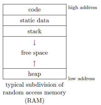
Now, we can address general issues of mapping high-level programming language constructs onto low-level features of the target machine. These issues include: data representation, mapping language values to words, bytes and bits; memory organisation, subdivision of RAM for code, static data, the stack and the heap; and the procedure call protocol, subdivision of work between the caller and the callee.
Data Representations
One form of data representation is constant-size, where all values of a type occupy the same amount of space, and knowing the type of the variable means knowing the space required for that variable.
These representations can either be direct, which is the binary representation itself (and allows for more efficient access) or indirect, which is a pointer to the actual representation. With indirect representations, pointers are always constant size, even if the type is not or is unknown (e.g., subtyping, polymorphism), and copying (argument passing) of the pointer is efficient.
Some basic types include booleans, which are one word, byte, or at it's smallest, a single bit: 0 (False) and 1 (True); characters, which are 1 or 2 bytes depending on whether it's an ASCII or Unicode representation; integers, which are a word (2 or 4 bytes depending on architecture) normally using two's complement representation is signed; floats, using the IEEE standard; and enumeration types (small integers).
More advanced types include records (or structs in C), which is a record composed of a list of fields, each referred to by an identifier and a field selection operator for accessing a specified field.
Fields are stored consecutively in memory, and the offset of each field is known at compile-time from the size of the preceeding fields, and the overall size of the record representation is known at compile-time.
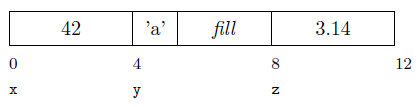
The address of a 2/4/8 byte value is normally a multiple of 2/4/8. On many machines this is either required, or yeilds faster memory access, therefore often unused fill is left between consecutive values. Reordering fields may reduce the internal fill, but this is sometimes forbidden by the language specification (such as in C).
Union types contain the value of only one of its components, and the operation is for accessing a specific component. All components have the same address, and the size of the union is the size of its biggest component. Unions introduce the danger of error in data interpretation, and many languages provide safe variants (e.g., variant records in Ada).
Arrays provide a mapping from a bounded range of indices to elements of one type, and an indexing operation is used for accessing an element of a given index. Elements are stored consecutively in memory with the memory address of a specific element given as: address(a[i]) = address(a) + i × size(typeof(a)). The value of i is usually only known at run-time, so we use run-time address computation.
Arrays bring further issues, however. For type safety, indexing code should check array bounds, and the first element may have an index unequal to 0. Multi-dimensional arrays are arrays of arrays, and you have to decide which array to consider first.
Another problem is that the array size may not be known at compile time, a lower bound is needed for indexing, and bounds are needed for a bound check. The bounds may be stored at the beginning of an array, and sometimes an indirect representation may be chosen for a constant size representation and simple copying.
Pointers are represented as the address of the value referred to, which means there is one machine-dependent size for all pointers. They are often needed for recursive types (lists, trees) or just indirect representation. The value referred to must be in RAM, not in a register.
Functions are often just represented as a pointer to the code entry point of the function, but more complex representations come up later.
Box/pointer diagrams are
around slide 75.
Classes are similar to records, but the method calls depends on the receiver object, so we also have a method table per class, with instance variables and methods at fixed offsets.
With inheritence, instance variables are inherited and new ones may be added. Methods are also inherited or overwritten and new ones may be added. Inherited/overwritten instance variables and methods are accessed at the same offsets. Indirect representation of objects is usually used to handle different sizes of direct representations.
Memory Organisation & Procedure Call Protocol
For global variables, static variables of cuntions and constants and literals that are not stored directly in the code (eg., printf("Hello world");), we can use static storage allocation, as a fixed address means efficient access.
Now we need to consider procedures (or functions, subroutines, methods, etc). If we consider simple recursive procedures without arguments and local variables, we have a program counter, which is the address of the next instruction to be executed, and at the end of procedure execution we need a return address (the address after the call instruction which passed control to the procedure). For arbitrarily recursive procedures, a stack of return addresses (corresponding to the nesting of the procedure calls) is needed.
If we consider a more advanced (and realistic) case of procedures with arguments and local variables, then each procedure activation has its own arguments and local variables with the same lifetime as the procedure is active for. Instead of a simple return address stack, we push a stack frame (sometimes called an activation record) onto the stack for each procedure call. When procedure execution completes, the frame is popped from the stack.
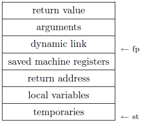
A typical stack frame is shown above. The global frame pointer (fp) points to the middle of the current frame on the stack, and all frame components (especially variables) are accessed by a fixed offset from fp. Sometimes, a global stack pointer (st) points to the top of the stack, and the dynamic link (sometimes called the control link) points to the preceeding frame on the stack (that is, the old value of fp). This is often only used because the frame size is not known until late in the compler phases.
The procedure call protocol defines the exact stack frame format and the division of work between the caller and the callee, e.g., the caller writes arguments, dynamic link, machine registers and return address to the frame and sets the new frame pointer, and the callee writes the return value and resets the fp.
The standard protocol is usually defined by OS and machine architecture, meaning it is not optimal for every language, but is needed for OS and foreign language calls.
How the arguments are passed also should be considered here. There are two types of argument passing mechanisms: pass by value and pass by reference. With pass by value, the argument is evaluated by the caller and the value passed to the callee. Update of the argument variable in the callee does not change an argument value in the caller. With pass by reference, the argument must be a variable (or any expression that has an address), and the address of tehv variable is passed (the l-value), thus an argument can be used to return a result.
With nested procedure definitions this becomes more complex, as we need to consider how to access a local variable or argument of the enclosing procedure. One solution is to add a static link (sometimes called an access link) to the frame of the inner procedure. Another solution is to use a global display - an array of frame pointers. An entry at index n points to a frame of nesting depth n. This allows faster access, and the maximal display size is the maximal nesting depth.
We should also consider procedures as arguments. How can a procedure that is passed as an argument access the variables or arguments of its enclosing procedures? The way to solve this is to represent a procedure as a pair of the entry point and the static link. The display technique is unsuitable, because the display is larger than one static link.
Something else to consider is procedures as results. How can a procedure that is returned as a result access the variables and arguments of its enclosing procedures? If we need the lifetime of arguments and local variables of a procedure longer than the procedure activation, we can not store them on the stack. In this casr then, arguments and local variables are stored on the heap, and garbage collection is used for deallocation after the end of the lifetime.
Access to registers is typically much faster than RAM, and modern CPUs have many (typically 32), divided into global registers (pc, fp, etc), caller-save registers and callee-save registers. Typically the procedure result is returned in the register, the first 4-6 procedure arguments are passed in to register and the caller stores the return address in a register. Registers may have to be spilled into a frame later, but many procedures do not call other procedures, and register values may only be needed before the first procedure call.
Heap
For data where the amount of size is not known at compile-time, or the lifetime is shorter than the whole program run-time, but not linked to procedure activation, we use dynamic memory, called the heap.
Allocation on the heap can either be explicit (e.g., malloc()) or implicit, where all values are heap allocated (e.g., Haskell). Similarly, deallocation can be explicit (e.g., free()), or implicit through garbage collection.
At run-time, the heap expands and occasionally contracts, and this deallocation usually leaves a gap. A run-time module called the heap manager maintains a free list, and this free list is a linked list of gaps.
Fragmentation occurs over time where gaps become smaller and more numerous. The total free space is large, but there is no single gap sufficient for an allocation. To combat this, we can allocate a best-fit instead of first-fit algorithm, coalesce adjacent gaps, or compact the heap by shifting all data (garbage collection).
Garbage Collection
Garbage is heap-allocated records unreachable by any chain of pointers from program variables. Garbage collection is the process of reclaiming memory occupied by garbage for new records.
Whether or not a record is "live" can be approximated by reachability.
Mark-and-Sweep Collection
In mark and sweep collection, all reachable records are marked using depth-first search, and then the entire heap is sweeped, collecting unmarked records into a linked list.
The cost of mark and sweep collection can be computed with C = (c1R + c2H) / (H - R), where R = the size of reachable data, H = the heap size and C is the eventual garbage-collection cost per allocated word.
If R ≈ H, then C is very large, but if R << H, C ≈ c2. After garbage collection, R and H are known. If R/H > 0.5, the heap should be grown.
This has problems as the DFS algorithm is recursive, and requires a stack proportional to the longest path in the graph. This may require a huge stack. The solution is to use the current field x.fi to point back to record t from which x was reached. Only a short integer done[x] is is needed in every record to indicate the current field.
See slide 98 for a
pseudocode implementation.
Reference Counting
In reference counting, each record has a reference counter, which counts the number of pointers pointing to the record. Before every assignment from x to y, the counter of x is decremented and the counter of y incremented. When the counter reaches 0, the record is added to the free list and the records x points to are also decremented.
This has a problem of circular references, where cycles of garbage all referring to each other can not be reclaimed, and the cost of incrementing and decrementing.
Copying Collection
The idea here is that the heap is divided into from-space and to-space, and that it starts with both reachable records and the garbage in the from-space, and then reachable records only in the to-space.
Copying is compact, fragmentation is eliminated, and allocation fron contiguous free memory is cheap.
Pseudocode for Cheney's
algorithm is in slide 101.
One algorithm that implements this idea of Cheney's breadth-first copying algorithm. The cost of this algorithm is C = c3R / (H/2 - R).
With the cost algorithm for Cheney and mark-and-sweep, we can plot the two to see in which case it is optimal to use which one:
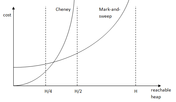
A problem with breadth-first copying is poor locality of reference (i.e., record pointing to another record that is located far from it). A good locality of reference improves memory access time, because of memory cache and virtual memory.
Depth-first copying provides a better locality of reference, but is more complicated (requiring pointer reversal). A solution is to use a hybrid of depth-first and breadth-first copying.
Generational Collection
We can observe that newly allocated records are likely to die soon, and older records are likely to live longer. Using this, we can divide the heap into generations, where G0 consists of the youngest records, and G1 consits of records older than the oldest in G0 and so on. Garbage collection then only needs to collect some generations, and records get promoted when it has survived 2-3 collection. Each generation is exponentially larger than the previous.
To do this collection, we can use any mark-and-sweep or copying collector. This has the problem of roots including pointers in other generations. However, pointers from old to new records are rare, and updates to newer records are rare. Using this, we can generate code to remember each updated record.
Incremental Collection
Another problem is the interruption of program execution for long periods of time by garbage collection, especially for interactive or real-time programs. One solution is to interleave garbage collection and program execution, but this has the danger of collection missing reachable records.
One solution to this is tricolour marking. Records are classified into three colours: white, not yet visited; grey, visited but children not yet examined; and black, visited and all children visisted. The invariant "no black record points to a white record" .
This causes additional work when program execution modifies the reachability graph. Two different approaches can be used: a write barrier algorithm, when program execution stores a white pointer in a black object, it colours the pointer grey; and a read barrier algorithm, when program execution reads a white pointer, it colours it grey (this may use the virtual memory fault handler).
Compilers can help for garbage collection. A collectior must find all pointers in heap-allocated records, so each record is started with a pointer to a data layout descriptor. Pointers must also be found in variables and temporaries (especially on the stack and in registers). The use of temporaries changes continuously, and this information is only needed at function call (allocation call). One way to implement this is to have a mapping from the return address in the frame to the data layour descriptor.
Conservative collectors work mostly without compiler support by guessing what is a pointer.
Intermediate Languages
Intermediate languages exist to provide an interface between several front and back ends, and to allow reuse of the optimisation phase.
Intermediate languages have a number of desirable attributes, including independence of the source and target language, each construct having a clear and simple meaning (making it suitable for optimisation), as well as being easy to translate to and from the source languages.
These simple languages typically have few control structures (for example, only conditional jump and procedure calls), and no structured data types (only basic types and addresses), which means that explicit address computation and memory access is needed.
Sometimes compilers have several intermediate languages.
Intermediate languages fall into three classes:
- Tree or directed acyclic graph based languages are close to the source language, but are more simple, and are good for high-level optimisations;
- Stack-based languages are where all instructions obtain operands from, and return results to, the stack;
- Three-address instruction languages are useful for RISC-like machines with an unlimited number of registers.
Examples are around
slide 112 of the notes.
Evaluating expressions in a stack-based language results in code corresponding to the postfix representation of expression. Function calls are integrated with a procedure call, where arguments are pushed onto the stack, and the result is on top of the stack.
In three-address instruction languages, temporaries are the variables of the intermedite language, and all operations only work on temporaries, like registers in the RISC machine. The variables of the source code do not exist in the intermediate code.
The three-address instruction language from the notes (and the one we will undoubtedly need to learn) has only a single type for integers, booleans and addresses, otherwise different move instructions and possibly different temporaries would be needed.
a ← b binop c- operation on temporariesa ← M[b]- move from memoryM[a] ← b- move to memorya ← b- move between temporariesL:- mark code address with labelLgoto L- jump to labelLif a relop b goto L- conditional jumpf(a1, ..., an)- procedure callb ← f(a1, ..., an)- procedure call with return valueenter f- beginning of procedurereturn- end a procedurereturn a- end a procedure that has a return value
a, b and c are temporaries or constants, and L and f are labels.
Both stack-based and three-address instruction languages yield linear programs (a sequence of instructions. Stack-based generally leads to fewer addresses and compact code, and does not need later register allocation like three-address code. Three-address code, however, profits from fast registers whereas stack-based code does not, and three-address instructions are easier to rearrange than stack instructions, so three-address code is easier to optimise than stack code.
Intermediate Code Generation
It is important to remember that only the intermediate language is target language independent, and the intermediate code contains addresses and offsets, which is target machine specific. For portability, all address computation should be kept separate in code generation.
The intermediate code generation phase therefore has two main parts: storeage allocation, which fixes addresses or offsets for each variable identifier (memory organisation), where the address or offset is a target machine specific attribute of an identifer (the identification phase should ensure that this attribute is shared by all occurrences of the same identifier and this attribute should be written when processing the declaration; and the actual translation to intermediate code.
There are two ways to implement the translation which fall under the definition of "syntax-directed" translation: specification by synthesised attribute, where intermediate code generation can be viewed as an attribute computation similar to many of the attribute problems discussed earlier; and specification by translation, where translation or compilation functions are used.
We can have expressions other than simple identifiers on the left-hand-side of assignments, so expressions on the left-hand-side need to be translated. We get l-values - the value of an expression that appears on the left-hand-side of an assignment (i.e., an address) and the value of an expression that appears on the right-hand-side of an assignment (e.g., the memory content at an address). Different translations for the expressions are required, one for l-value (transLExp) and one for the r-value (transExp). Not all expressions may be on the lhs, so transLExp may not be defined for all expressions.
Slide 121 onwards contain
sample translation functions.
When translating operator expressions, the order of operand evaluation matters if the evaluation causes side effects. Operand evaluation order may be specified by the language (this is not the case in C, however). The sample function given assumes that op exists also in the intermediate language.
Structured control constructs (e.g., if) gets translated into (conditional) jumps. Some structures (such as while loops) can be translated in two different ways, which are sometimes more efficient depending on the context (e.g., one translation uses less instructions overall if there are multiple loops).
Most machines and intermediate languages do not support the boolean type directly, so False is represented as 0 and True as a 1. The result of relational operators can only be used in a conditional jump. Boolean operators can also be short circuited: a and b ⇒ if a then b else False, and a or b as if a then True else b.
Similarly, procedure calls depend on an argument evaluation order. The intermediate language must make sure it specifies the requirements of the procedure call protocol. The function identifier is used as a label, and the code for nested procedures is not nested.
Target Code Generation
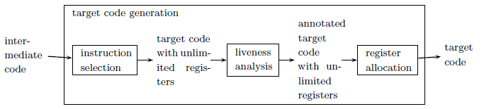
The target code might be assembly code, relocatable machine code, or absolute machine code, and may be for different architecutres including RISC or CISC machines.
Three-address instructions are even more primitive than RISC instructions, so translating each three-address instruction (after optimisation) separately yields inefficient code. It is necessary to combine several three-address instructions into one target instruction.
Generation is therefore done in two steps, first by translating three-address code into tree-based code by inlining of used-once-only definitions of temporaries, and then the tree-based code is translated into target code with an unlimited number of registers by tiling each tree with target code instructions.
To translate into a tree-based language, you must first locate definitions of temporaries that are used only once (that is, there is no redefinition, label, jump or call between definition and use) and these definitions are inlined at the use occurrence.
For some sample patterns,
see slide 133.
Target instructions are expressed as fragments of an intermediate code tree, called a tree pattern. Instructions can usually correspond to more than one tree pattern - this is called a tiling.
As usually several different tilings are possible, then each kind of instruction is assigned a cost. The optimum tiling is a tiling with the lowest possible costs, and an optimal timing is where no two adjacent tiles are combinable into a single tile of lower cost.
Optimum implies optimal, but this is not a transitive relationship.
In RISC architectures, instructions are typically all simple with a uniform cost, so there is little difference between the cost of optimum and optimal tiling. For CISC machines, the complex instructions have different costs, and there is a noticeable difference between the cost of optimum and optimal tiling.
The Maximal Munch tiling algorithm is a top-down algorithm that yeilds an optimal tiling. The algorithm starts at the root of a tree, finding the largest tile that fits. That tile covers the root node and some other nodes, leaving subtrees, and the algorithm is repeated for each subtree.
The Dynamic Programming tiling algorithm is bottom-up and yields an optimum tiling. The algorithm here is to assign to each a subtree and optimum tiling and the cost of that tiling computed by considering each tile that matches at the root. The cost of using a tile is the cost of the tile plus the costs of the optimum tiling of the remaining subtrees. The tile chosen is where the cost (as defined above) is minimal.
The grammar is
on slide 127.
Tiling can be considered parsing with respect to a highly ambiguous context-free tree grammar.
Tools that generate code generators process grammars that specify machine instruction sets, and associated with each rule of the grammar is a cost and action (or attribute equation).
Compilation functions can be used for a direct translation from the abstract syntax tree to target code, but this often leads to inefficient code, so these compilation functions are extended by special cases. The compilation functions is then based on overlapping tree patterns, so a tiling algorithm can be used for code generation.
Another problem is that when generating machine code, absolute or relative code locations have to be used instead of labels, which causes problems when addresses for forward jumps need to be generated. One option is to leave a gap in the code and add the jump later - this is called backpatching. You can either backpatch when the target location is known, or in a separate pass. A problem however is that shorter machine instructions are often used for shorter jumps.
Liveness Analysis & Register Allocation
Two temporaries can fit in the same register, as long as they are never live at the same time. A temporary is live if it holds a value that will be used in the future.
A process known as liveness analysis yiels a conservative approximation of liveness (static liveness). If the temporary is live, then the analysis will say so, but it does give false positives - if the analysis says the temporary is live, this does not necessarily mean so.
Two analysis methods include data flow analysis, where liveness is determined by the flow of data through the program; and backwards analysis, from the future to the past.
In general, liveness analysis and register allocation is only for one procedure body at a time. It is easier to use three-address code rather than specific target code to do this analysis.
For examples, see
slide 142.
A control flow graph can be built, where nodes are the instructions of the program (excluding labels), and an edge exists from x to y if the instruction x can be followed by instruction y.
The control flow graph is an approximation of dynamic control flow.
- out-edges of a node n lead to successor nodes: succ(n);
- in-edges of a node n come from predecessor nodes: pred(n);
- def(n) is a set of temporaries defined by an instruction at node n;
- use(n) is a set of temporaries used by an instruction at node n;
- A temporary t is live on an edge e iff there exists a path from e to a use of t that does not go through a definition of t;
- in(n) is a set of temporaries that are live on any in-edge of n;
- out(n) is a set of temporaries that live on any out-edge of n.
We can more formally define in(n) and out(n) as:
- in(n) = use(n) ∪ (out(n) \ def(n))
- out(n) = ∪s ∈ succ(n) in(s)
The algorithm for liveness is then as follows:
foreach n:

      in(n) := ∅

      out(n) := ∅

  repeat

      foreach n:

          in′(n) := in(n)

          out′(n) := out(n)

          out(n) := ∪s ∈ succ(n) in(s)

          in(n) = use(n) ∪ (out(n) \ def(n))

  until in′(n) = in(n) and out′(n) = out(n) for all n
The run time for this algorithm is better if nodes are processed approximately in the reverse direction of control flow. In the worst case it is Ο(N$), but in practice it tends to lie between Ο(N2) and Ο(N4) (where N is the number of nodes).
Another thing to consider for register allocation is an interference graph, where nodes are temporaries, and edges are interferences (temporaries that can not be allocated to the same register). All temporaries in the same live-in or live-out set interfere, with the extra case of a temporary t defined by the instruction t ← ... shall always be in the live-out set of instructions, even if not actually live-out.
Slide 146 contains the
graph colouring algorithm.
Mapping these temporaries to K registers saves memory access time. To compute the registers, the interference graph needs to be K-coloured. This is NP-complete, so the approximation algorithm should be used. If K-colouring is impossible, than some temporaries get spilled over into memory.
Assignments such as t ← s do not make an interference edge between t and s, because they can be mapped to the same register. We can therefore coalesce nodes t and s in the interference graph and delete the instruction t ← s.
However, coalescing can hinder K-coloring, so we should only coalesce if the resulting node has fewer than K neighbours. This coalescing needs to be integrated into the K-colouring algorithm (as the number of neighbours change), and the preceeding compiler phases are therefore free to insert move instructions where convenient.
We also need to aim to minimise the number of stack frame locations for spilled temporaries, and the number of move instructions involving pairs of spilled temporaries. Hence, we should construct an interference graph for spilled nodes, and coalesce aggressively (as the number of stack frame locations is not limited) and finally colour the graph.
Sometimes it is necessary to have a register in the interference graph as a pre-coloured node, and all pre-colour nodes interfere with each other. We can express that some temporaries have to be in specific registers (e.g., the frame pointer), or that some instructions only work with certain registers. Also, call instruction invaldiates all caller save registers (the callee save registers used for temporaries live across procedure call), and the register allocator ensures saving of caller save registers.
Optimisation
Optimisation takes intermediate code and returns optimised code. It is important to note that optimisation does not yield optimal code. The requirements of optimisation are to preserve the meaning of the program (including errors), to on average improve the program (mostly runtime, but sometimes space and program size) and is worth the cost (optimisation can be complex and extends compile time).
Programs should be modular and easy to understand, and many optimisations need access to low-level details inaccessible to high-level languages (e.g., addressing), so it is often better to have the compiler do optimisations, not the programmer. Additionally, ome optimisations use target machine specific knowledge, so the compiler can optimise for different target machines which if done in code would eliminate portability. However, optimisations are no substitute for good algorithm selection.
Optimisations done in the compiler can often lead to simple code generation.
Optimisation phases typically consist of a series of optimisations.
Optimisations for Eliminating Unnecessary Computations
The general gist of this is to do at compile time what would otherwise be done at run time. This can stretch from simple constant folding (if the operands of an instruction are constant, the computation can be done at compile time) to state-of-the-art partial evaluation/program specialisation (a whole program together with partial input data is transformed into a specialised version of the program by precomputing parts that depend only on that specific input data).
An example of program specialisation is compiling interpreted core - the interpreter is specialised with respect to the input program.
Arithmetic identities can be used to delete superfluous operations (e.g., t1 ← t2 * 1 to t1 ← t2).
Dead code (code that can never be reached) can be eliminated, and instructions which compute values that are never used can also be.
Array bound checks can also be eliminated, as often the compiler can determine if the value of an index variable is always within the array bounds.
Induction variables can also be eliminated. Some loops have a variable i which is just incremented or decremented, and a variable j that is then set to i × c + d, where c and d are loop-invariant. j's value can then be calculated without reference to i, and whenever i is incremented, we can just incrememnt j by c.
Common subexpressions from multiple expressions can be eliminated by computing it only once, then saving the value and using it whereever needed. Many common subexpressions are actually compiler-generated address calculations.
Code motion can also be done, ranging from hoistnig loop-invariant computations (moving instructions that compute loop-invariant values out of a loop) to lazy code motion (moving all instructions as far up in the control-flow graph as possible, exposing exposes the maximum number of redundancies and instructions are pushed as far down in the control-flow graph as possible, minimising register lifetimes).
Optimisations for Reducing Costs
These optimisations include reduction in strength, replacing expensive instructions with cheaper ones (e.g., t1 ← t1 * 4 to t1 ← t1 << 2).
Replacing procedure calls with the code of the procedure body (inlining) can also be an optimisation. Here, the procedure parameters are also replaced in the instruction arguments.
Modern computers can execute parts of many different functions at the same time, but dependencies between instructions hinder this instruction-level parallelism, so by reordering instructions to minimise dependencies, we can optimise instruction scheduling.
Aligning and ordering instructions for data so they are mapped efficiently into cache can speed up memory access (cache being must faster than main memory, but also much slower). By using this cache-aware data access, we can also ensure that data structure traversals (especialyl of arrays) take advantage of the cache.
Enabling Optimisations
Optimisations in this class don't themselves result in optimisations, but they enable applications of other optimisations.
Constant propagation can be used when the value of a temporary is known to be a constant at an instruction, so the temproary can simply be replaced by the constant.
Copy propagation is similar, but instead of a constant there is a temporary (similar to coalescing in register allocation).
Loop unrolling can be used to put two or more copies of a loop body in a row.
Optimisations are typically applied to intermediate code to enable reuse in different front and back ends, however some optimisations are most easily expressed on a different program representation (closer to the source or target code), and some optimisations are target code specific (special machine instructions).
Determining a sequence of optimisations is complex because each optimisation uncovers opportunities for other optimisations, and the effects of many optimisations overlap, with some subsuming others.
A basic block is a maximal-length sequence of three-address instuctions that is always entered at the beginning and is exited at the end. That is, a label may only appear as the first instruction, and a jump may only appear as the last instruction.
To prepare for optimisations, the code is divided into these basic blocks and a control-flow graph is built of the basic blocks.
Locality
Optimisations can also be classed with regard to locality.
A peephole optimisation slides a several instruction window over the target code, looking for a suboptimal pattern of instructions. Constant folding and strength reduction falls into this class.
Local optimisations operate on single basic block.
Global (or intraprocedural) optimisations operate on procedure bodies. All loop optimisations fall into this class.
Interprocedural optimisations operate on several procedure bodies. Procedure inlining and partial evaluation fall into this class.
Many optimisations can be performec, with different effectiveness, on either a peephole, local, global or interprocedural level.
The runtime of many optimisation algorithms is not linear, but often quadratic or worse.
Most optimisations require information from an analysis.
Dead code can be detected as any instruction which assigns to a variable a and a is not live-out of the instruction, and the instruction can not cause a side effect (e.g., arithmetic overflow, or division by zero).
Reaching Definitions
Slide 162 onwards contains
a reaching definition algorithm.
A definition of a temporary t is a control-flow node where it is assigned something, we can say that a definition d of t reaches a control-flow node n if there is a path from d to n without any definition of t. Several definitions of t may reach a node, because the control flow graph approximates dynamic control flow.
For the actual applications,
see slides 165 onwards.
If d reaches n and no other definition of t reaches n, then we can apply constant propagation.
If d reaches n, no other definition of t reaches n and no definition of z on any path from d to n, we can apply copy propagation.
Forward substitution can be done on associative operators, if d reaches n, no other definition of t1 reaches n and there is no defintion of r on any path between d and n.
Common subexpression elimination can be applied if the right-hand-side of d equals the right-hand-side of n, d reaches n, no other definition of t1 reaches n and there is no definition of r on any path between d and n.
Dead code elimination can be applied if d1 reaches no node that uses t.
Data flow analysis can be done using liveness or reaching definitions. Liveness uses backwards analysis, and reaching definitions uses forward analysis. Equations may have more than one solution, but Knaster-Tarski fixpoint theorem states that the least solution is the start with empty sets and add elements.